UNet is a winner of the ISBI bioimage segmentation challenge 2015.
It relies on data augmentation to use the available annotated samples more efficiently.
The architecture consists of a contracting path to capture context
and a symmetric expanding path that enables precise localization.
This application is being used as a biological example in class #1 of the course
"Deep Learning by Example on Biowulf".
Allocate an interactive session and run the program. Sample session:
[user@biowulf]$ sinteractive --mem=16g --gres=gpu:v100:1,lscratch:10 -c4
[user@cn4471 ~]$module load unet
[+] Loading cuDNN/8.0.3/CUDA-11.0 libraries...
[+] Loading CUDA Toolkit  11.0.3  ...
[+] Loading gcc 4.8.5  ...
[+] Loading Qt 5.9.4  ...
[+] Loading UNet 20210223  ...
The bin directory of the application includes three executable files: train.py, predict.py and visualize.py. In order to display the usage message and available command line options for an executable, type its name followed by the option "-h". For example:
[user@cn4471 ~]$ train.py -h
...
usage: train.py [-h] -d data_folder [-a augmentation_rate] [-b batch_size] [--beta tversky_beta] [-c object_class]
                [--cw class_weights] [--drop_rate drop_rate] [-e num_epochs] [-F start_filters] [-g num_gpus]
                [--gamma tversky_gamma] [-l learning_rate] [--loss loss_type] [-n] [-s] [--save_augmented] [-v]
                [-w] [-X X] [-Y Y]

optional arguments:
  -h, --help            show this help message and exit
  -a augmentation_rate, --augmentation_rate augmentation_rate
                        by how many folds to increase the effective data size; default=20
  -b batch_size, --bs batch_size
                        batch size; default=2
  --beta tversky_beta   class balancing weight in the Trersky index: TI = TP/(TP + beta*FP + (1-beta)*FN)
  -c object_class, --object_class object_class
                        Detected object class(es): memb | mito | multi; default = membr
  --cw class_weights    Comma-separated class weights
  --drop_rate drop_rate
                        drop rate; default=0.5
  -e num_epochs, --num_epochs num_epochs
                        number of epochs; default=160
  -F start_filters, --start_filters start_filters
                        num. filters used in the 1st convolution of the network model; default=64 if
                        object_class=membr; =8 if object_class=mito; and =48 if object_class=multi
  -g num_gpus, --num_gpus num_gpus
                        number of gpus to use; default=1
  --gamma tversky_gamma
                        a power in the Trersky focal loss
  -l learning_rate, --lr learning_rate
                        learning rate; default=1.e-4
  --loss loss_type      loss type: bce | cce | wcce | dice | jaccard | tversky; default: wcce if object_class ==
                        'multi' and bce otherwise
  -n, --no_augmentation
                        don't perform data augmentation, i.e. use original input data; default=False
  -s, --summary         print the model summary
  --save_augmented      save augmented data (in the subfolder 'augmented'
  -v, --verbose         increase the verbosity level of output
  -w, --load_weights    read weights from a checkpoint file
  -X X, --image_width X
                        image width; should be multiple of 16; default=256
  -Y Y, --image_height Y
                        image height; should be multiple of 16; default=256

required arguments:
  -d data_folder, --data_folder data_folder
                        data folder name, e.g. 'data_isbi' or 'data_hhmi'
In order to run the training executable on available sample data, first compy the data to your current folder:
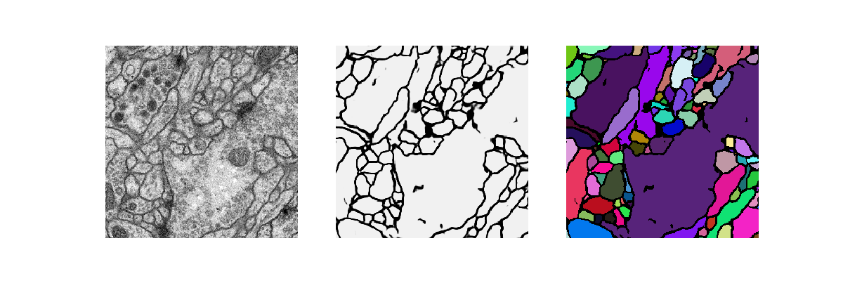
[user@cn4471 ~]$ cp -r $UNET_DATA/* .There are currently two sample datasets available, both comprising 2D EM images of Drosophila brain slices. The first dataset includes 30 pre-processed grayscale images together with corresponding binary masks for neural membranes from the ISBI Challenge. It comes together with the Keras UNet implementation code available at GitHub. This dataset is stored in the folder "data_isbi".
[user@cn4471 ~]$ train.py -d data_isbi
Using Tensorflow backend.
...
Epoch 1/100
300/300 [==============================] - 28s 92ms/step - loss: 0.6890 - acc: 0.7793
Epoch 2/100
300/300 [==============================] - 21s 71ms/step - loss: 0.6809 - acc: 0.7817
Epoch 3/100
300/300 [==============================] - 21s 71ms/step - loss: 0.6731 - acc: 0.7815
Epoch 4/100
...
Epoch 99/100
300/300 [==============================] - 21s 71ms/step - loss: 0.0979 - acc: 0.9765
Epoch 100/100
300/300 [==============================] - 21s 71ms/step - loss: 0.0965 - acc: 0.9766
The trainig results, i.e. model weights, will be stored in the checkpoint file stored in the folder "checkpoints", in the HDF5 format,
checkpoints/<model_name>.<data_folder_name>.<object_class>.h5in this particular case - in the file:
checkpoints/unet.data_isbi.membr.h5.The prefix of the output checkpoint file can be changed through a command line option of the train.py.
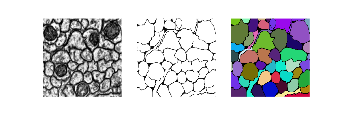
[user@cn4471 ~]$ predict.py -d data_isbi
Using TensorFlow backend.
...
30/30 [==============================] - 2s 81ms/step
...
For each the grayscale image file i.png (i=0,1,...,29), this command will produce a binary mask i_predict.png together with an RGB image i_predict_RGB.png with colored the connected components of the binary image.
[user@cn4471 ~]$ visualize.py -h
usage: visualize.py [-h] [-c object_class] [-d data_folder] [-i image_path] [-n image_id]

optional arguments:
  -h, --help            show this help message and exit
  -c object_class, --object_class object_class
                        Detected object class(es): membr | mito | multi; default = membr
  -d data_folder, --data_folder data_folder
                        path to the top data folder
  -i image_path, --image image_path
                        a path to the image to be visualized
  -n image_id, --image_id image_id
                        a number in the range(num_images)
Here, either the option -i or -n is required. For example, to visualize the 0-th data item, type:
[user@cn4471 ~]$ visualize.py -n 0 -d data_isbi
[user@cn4471 ~]$ train.py -d data_hhmi
Using TensorFlow backend.
...
Epoch 1/100
300/300 [==============================] - 31s 104ms/step - loss: 0.1928 - acc: 0.9111
Epoch 2/100
300/300 [==============================] - 22s 72ms/step - loss: 0.1388 - acc: 0.9335
Epoch 3/100
300/300 [==============================] - 21s 71ms/step - loss: 0.1269 - acc: 0.9395
...
Epoch 159/160
240/240 [==============================] - 17s 72ms/step - loss: 0.0351 - acc: 0.9856
Epoch 160/160
240/240 [==============================] - 17s 72ms/step - loss: 0.0349 - acc: 0.9856
This command will produce a checkpoint file hhmi.membrane.h5 in folder "checkpoints".
[user@cn4471 ~]$ cp -r $UNET_DATA/checkpoints .Now we can run the executable predict.py:
[user@cn4471 ~]$ predict.py -d data_hhmi
Using TensorFlow backend
...
24/24 [==============================] - 2s 98ms/step
...
[user@cn4471 ~]$ visualize.py -n 1 -d data_hhmi
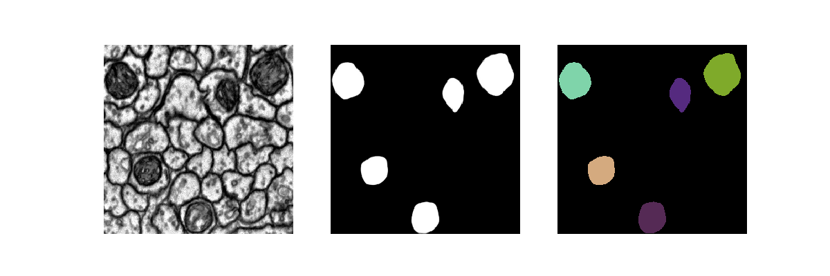
[user@cn4471 ~]$ train.py -d data_hhmi -c mito
...
[user@cn4471 ~]$ predict.py -d data_hhmi -c mito
...
[user@cn4471 ~]$ visualize.py -n 1 -d data_hhmi -c mito
[user@cn4471 ~]$ exit
[user@biowulf ~] sinteractive --mem=16g --gres=gpu:v100:4,lscratch:40 -c14
[user@cn4471 ~]$ module load unet
[user@cn4471 ~]$ cp -r $UNET_DATA/* .
[user@cn4471 ~]$ train.py -d data_isbi -g 4 -b 8
Using TensorFlow backend.
...
 StreamExecutor with strength 1 edge matrix:
2019-04-23 07:38:17.419226: I tensorflow/core/common_runtime/gpu/gpu_device.cc:988]      0 1 2 3
2019-04-23 07:38:17.419241: I tensorflow/core/common_runtime/gpu/gpu_device.cc:1001] 0:   N Y N N
2019-04-23 07:38:17.419252: I tensorflow/core/common_runtime/gpu/gpu_device.cc:1001] 1:   Y N N N
2019-04-23 07:38:17.419262: I tensorflow/core/common_runtime/gpu/gpu_device.cc:1001] 2:   N N N Y
2019-04-23 07:38:17.419271: I tensorflow/core/common_runtime/gpu/gpu_device.cc:1001] 3:   N N Y N
...
Epoch 1/160
18/18 [==============================] - 28s 2s/step - loss: 0.6806 - acc: 0.7497
Epoch 2/160
18/18 [==============================] - 11s 588ms/step - loss: 0.5285 - acc: 0.7811
Epoch 3/160
18/18 [==============================] - 11s 590ms/step - loss: 0.4687 - acc: 0.7814
...
End the interactive session:
[user@cn4471 ~]$ exit
salloc.exe: Relinquishing job allocation 46116226
[user@biowulf ~]$
Create a batch input file (e.g. unet.sh). For example:
#!/bin/bash
module load unet
cp -r $UNET_DATA/* .
train.py  -e 100 -l 0.0001
Submit this job using the Slurm sbatch command.
sbatch [--cpus-per-task=#] [--mem=#] unet.sh