Chapter 1 Data preprocessing

1.1 Brief introduction

Data preprocessing includes read trimming, alignment, sorting by coordinate, and marking duplicates. Duplicate marking itself is discussed in Chapter 3. GATK’s duplicate marking tools perform more efficiently with queryname-grouped input as generated by the aligner and produce sorted BAM output so the most efficient pipeline would not write sorted BAM files from the aligner. However, in other cases a sorted BAM file prior to marking duplicates may be desired. Therefore, in this Chapter benchmarks and scripts for either unmodified or sorted BAM output from FASTQ files are presented.

For efficiency trimming, alignment, and converting (or sorting) to BAM format are run concurrently with data flowing through linux pipes to avoid unnecessary IO. The thoughput of each of the three components should be similar to each other and within the range of good parallel efficiency (70~80% of ideal performance).

Whether sorting or not, it is important to not write uncompressed SAM files to disk since conversion to BAM is not computationally intensive and BAM files are much smaller than SAM files.

Note that the GATK best practices pipeline starts from an unaligned BAM file (ubam) and includes some additional steps but for the purposes of this tutorial these are omitted.

1.2 Tools

fastp 0.20.1
bwa 0.7.17
samtools 1.11
mosdepth 0.3.0

1.3 Individual tool benchmarks

First we optimize each individual step.

1.3.1 Adapter trimming

While we use fastp for this step, there are many other ways of trimming adapters. In this Section read pairs are written interleaved to stdout and discarded because in the later preprocessing Section 1.4.2 read pairs will be piped directly to bwa to avoid unnecessarily writing temporary data to disk. FASTQ files were read from lscratch to avoid inconsistent results due to file system load and all tests were run on x2695 nodes. The command used was:

fastp -i /lscratch/${SLURM_JOB_ID}/$(basename $r1) \
     -I /lscratch/${SLURM_JOB_ID}/$(basename $r2) \
     --stdout --thread $threads \
     -j "${logs}/fastp-${SLURM_JOB_ID}.json" \
     -h "${logs}/fastp-${SLURM_JOB_ID}.html" \
     > /dev/null

This will use the default quality filters and remove adapters based on pair overlap. Other filters may reduce throughput.

Figure 1.1 shows that fastp is fast but parallel efficiency quickly drops beyond 6 threads. Therefore fastp should be limited to no more than 6 threads. See table 1.1 for a summary of throughput and efficiency.

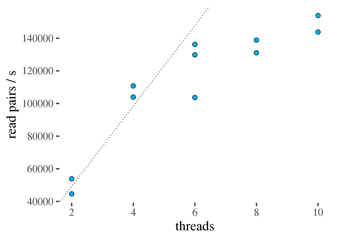
Figure 1.1: Throughput of fastp in read pairs per second as a function of the number of threads. Ideal scaling is shown as a dotted line.

Table 1.1: fastp efficiency
threads	Efficiency [%]	pairs/s
2	100	49243
4	109	107353
6	83	123228
8	69	134955
10	60	148827

1.3.2 Alignment

In this Section standalone bwa is used to produce the primary alignment. For the benchmark, bwa is fed separate FASTQ files from lscratch and outputs SAM format alignments to /dev/null. In the pipeline from later Section 1.4.2 it will ingest interleaved trimmed reads from fastp and output directly to samtools. Here is the bwa command used in the benchmarks:

bwa mem -M -t ${threads} \
        -R "@RG\tID:$id\tPL:ILLUMINA\tLB:$lb\tSM:$sm" \
        $genome \
        /lscratch/$SLURM_JOBID/$(basename ${r1[small]}) \
        /lscratch/$SLURM_JOBID/$(basename ${r2[small]}) \
        > /dev/null

Note that the content of the read group (@RG) SAM header field will be discussed in Section 1.5.

As for fastp all benchmarks were run on x2695 nodes. Figure 1.2 shows the scaling of bwa with increasing numbers of threads. bwa scales well to 32 threads (table 1.2). Even though bwa scales much better than fastp but it does much more computing per read pair it process much less reads per second than fastp. That means theoretically 2 threads of fastp (49243 pairs/s) are sufficient to feed 32 threads of bwa (22087 pairs/s).

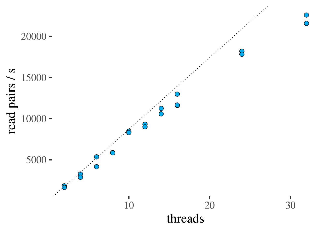
Figure 1.2: Throughput of bwa in read pairs per second as a function of the number of threads. Ideal scaling is shown as a dotted line.

Table 1.2: BWA efficiency
threads	Efficiency [%]	pairs/s
2	100	1741
4	89	3087
6	91	4761
8	84	5865
10	96	8392
12	88	9167
14	90	10915
16	87	12085
24	86	18009
32	79	22087

1.3.3 Alternative A: Sorting by coordinate

In the later alignment script @ref({#preproc-view}, the SAM output of bwa will be piped directly into samtools to avoid unnecessary writes to disk. However, to test samtools sort scaling in this Section, we use an unsorted BAM file as input. Not ideal but it will give us a good idea of samtools throughput and scaling. Note that samtools needs to spill temporary files to disk if the alignment does not fit in memory which will generally be the case for whole genome alignments. To improve performance and avoid unnecessary load on the shared file systems, it is very important to use lscratch for these temporary files.

The samtools command in the tests:

samtools sort -T /lscratch/$SLURM_JOBID/part \
    -m ${mem_mb_per_thread}M \
    -@ ${threads} \
    -O BAM \
    /lscratch/$SLURM_JOBID/$(basename $bam) \
     > /dev/null

Notes:

The input BAM file was 32GB located in lscratch.
Temporary files were stored in lscratch.
Output was discarded.
For these benchmarks the sort was run with different amount of total memory (10GiB, 20GiB, and 30GiB) and different numbers of threads.
The amount of temporary space on lscratch used was about 1.5x that of the input BAM file and 1.75x that of the input compressed FASTQ files.
The job was allocated about 5GB more memory than threads * mem_per_thread to avoid out of memory kills (i.e. 15GB, etc.).

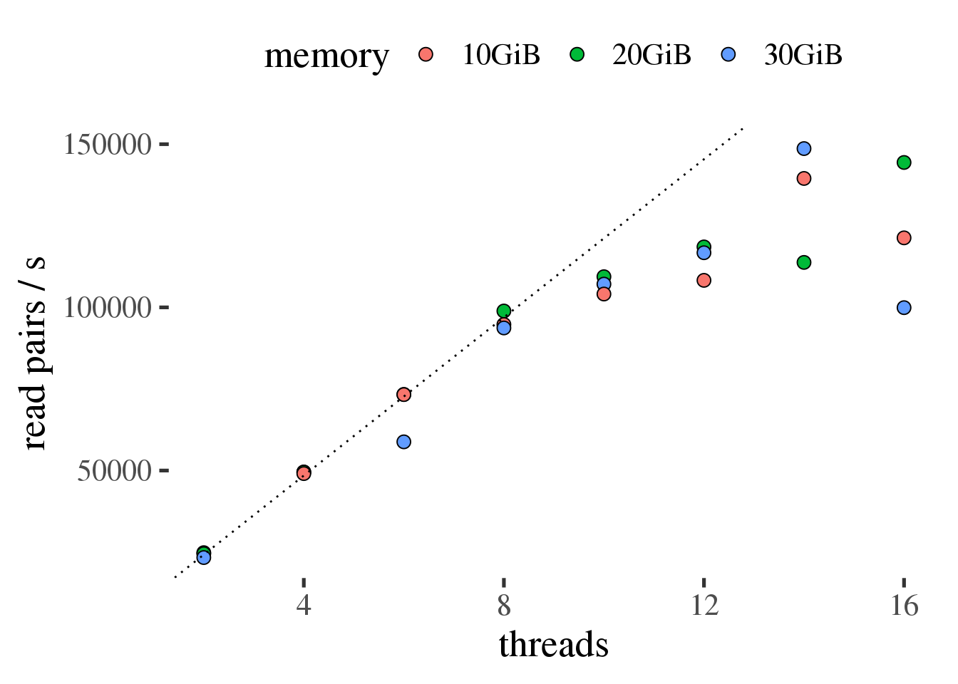
Figure 1.3: Throughput of samtools sort in read pairs per second as a function of the number of threads. Ideal scaling is shown as a dotted line.

Figure 1.3 shows that samtools sort scales efficiently up to 10 threads in this test and that the amount of total memory across all threads did not result in measurably different performance.

Table 1.3: samtools efficiency
threads	Efficiency [%]	pairs/s
2	100	24232
4	102	49383
6	94	68466
8	99	95778
10	88	106872
12	79	114514
14	79	133980
16	63	121872

1.3.4 Alternative B: Queryname-grouped (unsorted) BAM

In the later alignment script @ref({#preproc-view}, the SAM output of bwa will be piped directly into samtools to avoid unnecessary writes to disk. Unlike in 1.3.3 in this test the SAM file is converted to a BAM file without sorting (queries with the same name are grouped) for further processing as described in Chapter 3.

The samtools command in the tests:

samtools view -@ ${threads} \
    -O BAM \
    /lscratch/\$SLURM_JOBID/$(basename $sam) \
    > /dev/null

Notes:

The input SAM file was 29GB located in lscratch.
Output was discarded.
samtools view uses comparatively little memory, 4GB in the tests.

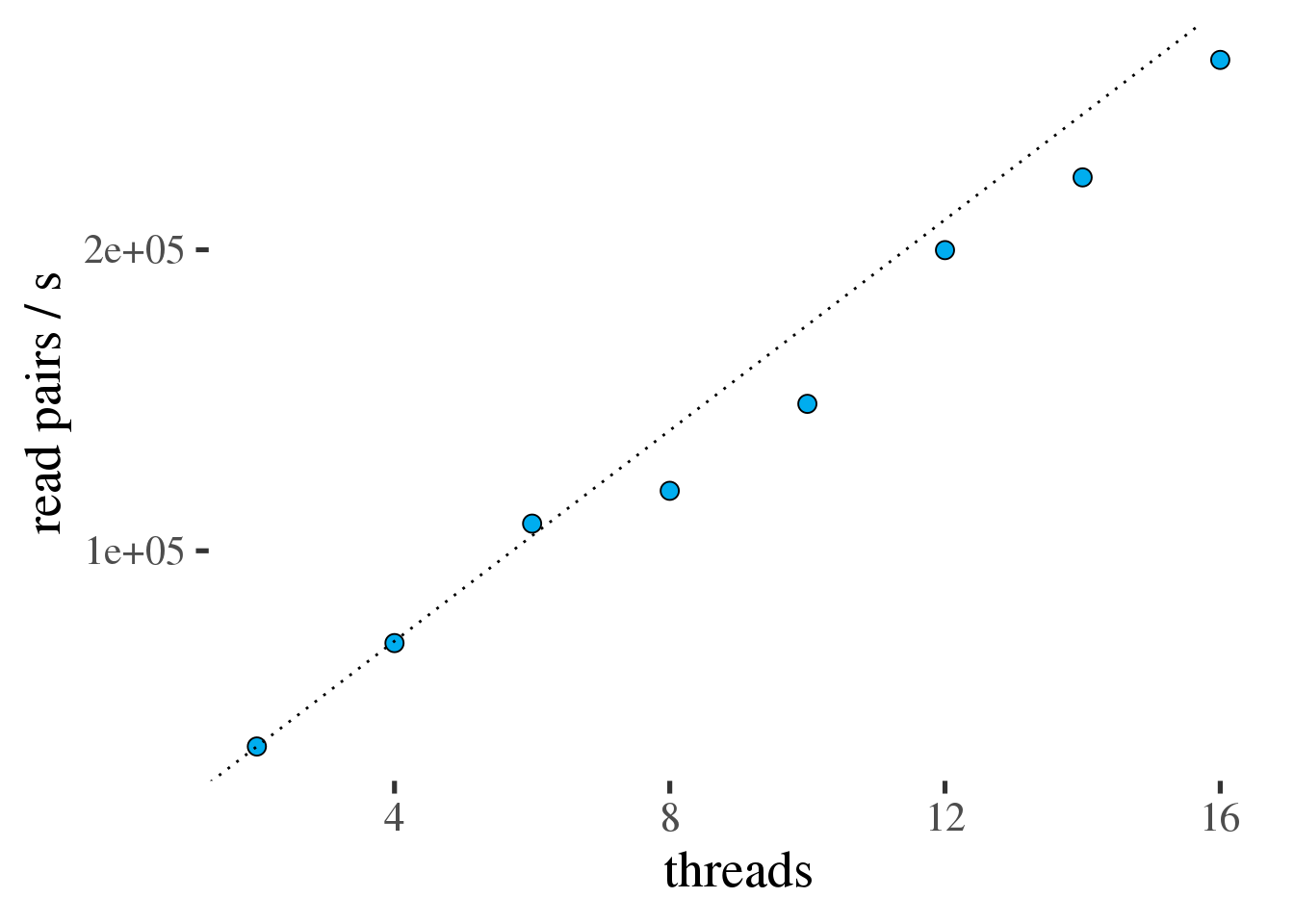
Figure 1.4: Throughput of samtools view in read pairs per second as a function of the number of threads. Ideal scaling is shown as a dotted line.

Figure 1.4 shows that samtools view scales efficiently all the way to 16 threads, the largest number of threads tested.

Table 1.4: samtools efficiency
threads	Efficiency [%]	pairs/s
2	100	35000
4	99	69346
6	104	109026
8	86	119928
10	85	148816
12	95	199880
14	91	224042
16	94	263068

1.4 Optimized script

Based on the individual benchmarks from Section 1.3 we can design an efficient combined pipeline with each tool running at > 80% parallel efficiency.

1.4.1 Alternative A: producing sorted BAM output

2 threads of fastp piping interleaved read pairs to bwa.
32 threads of bwa piping output.
12 threads of samtools with 20GB of memory; temporary files in lscratch.

In code:

fastp -i $read1 -I $read2 \
    --stdout --thread 2 \
    -j "${logs}/fastp-${SLURM_JOB_ID}.json" \
    -h "${logs}/fastp-${SLURM_JOB_ID}.html" \
    2> "${logs}/fastp-${SLURM_JOB_ID}.log" \
| bwa mem -v 2 -M -t 32 -p \
    -R "@RG\tID:$id\tPL:ILLUMINA\tLB:$lb\tSM:$sm" \
    $genome - 2> ${logs}/bwa-${SLURM_JOB_ID}.log \
| samtools sort -T /lscratch/$SLURM_JOBID/part \
    -m 1706M \
    -@ 12 \
    -O BAM \
    -o /lscratch/$SLURM_JOBID/$bam \
    2> ${logs}/samtools-${SLURM_JOB_ID}.log

For an input file with 201,726,334 read pairs we would expect a runtime of about 2.5h given the rate limits of ~22,000 pairs/sec in the alignment step. Since we are not sure about the total memory usage, we run this job with 46 CPUs and 70GB. Figure 1.5 shows the memory and CPU usage.

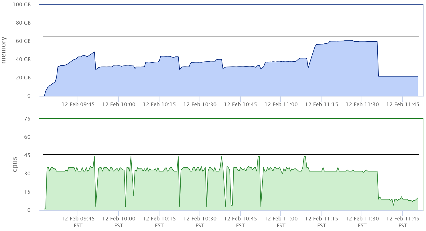
Figure 1.5: First implementation of combined preprocessing script

Some observations:

Memory usage peaked just above 60GB.
The code used only 32 CPUs most the time. This has to do with the fact that bwa and samtools don’t generally use lots of CPU at the same time. samtools accumulates alignments until its buffers are full and then sorts. While it sorts bwa will use less CPU.
The throughput of this run was similar to the throughput of bwa alone - about 20-24k read pairs per second.

The code above was run on 32 to 48 CPUs to see if throughput could be maintained at reduced core count. As can be seen in figure 1.6 (A) the throughput does increase linearly with the number of allocated CPUs from 32 to 48. However the increase is modest and efficiency, as measured in reads per second per CPU, decreases from 34 to 48 CPUs (figure 1.6 (B).

(A) Gross throughput in reads/s of the combined preprocessing pipeline from FASTQ to sorted alignments in a BAM file. The total thread count across all three tools. (B) Like the plot on the left but showing Reads/s/cpu, a measure of efficiency.

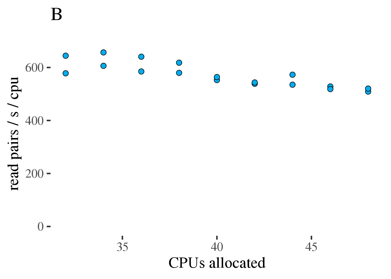
Figure 1.6: (A) Gross throughput in reads/s of the combined preprocessing pipeline from FASTQ to sorted alignments in a BAM file. The total thread count across all three tools. (B) Like the plot on the left but showing Reads/s/cpu, a measure of efficiency.

Based on this test we conclude that running the combined preprocessing steps with 46 threads on 34 CPUs is the most efficient approach and only results in a 12% increase of the runtime compared to 46 CPUs.

1.4.2 Alternative B: BAM output without coordinate sorting

2 threads of fastp piping interleaved read pairs to bwa.
32 threads of bwa piping output.
16 threads of samtools.

In code:

fastp -i $read1 -I $read2 \
    --stdout --thread 2 \
    -j "${logs}/fastp-${SLURM_JOB_ID}.json" \
    -h "${logs}/fastp-${SLURM_JOB_ID}.html" \
    2> "${logs}/fastp-${SLURM_JOB_ID}.log" \
| bwa mem -v 2 -M -t 32 -p \
    -R "@RG\tID:$id\tPL:ILLUMINA\tLB:$lb\tSM:$sm" \
    $genome - 2> ${logs}/bwa-${SLURM_JOB_ID}.log \
| samtools view -@ 16 \
        -O BAM \
        -o /lscratch/$SLURM_JOBID/$bam \
        2> ${logs}/samtools-${SLURM_JOB_ID}.log

For an input file with 201,726,334 read pairs we would expect a runtime of about 2.5h given the rate limits of ~22,000 pairs/sec in the alignment step. Some initial experiments showed that 42GB of memory were required for all test jobs to finish. As for alternative A we tested different numbers of CPUs - from a full allocation of 50 CPUs down to 32 CPUs to account for the fact that all three tools don’t operate at full capacity all the time.

As can be seen in figure 1.7 A the throughput does increase linearly with the number of allocated CPUs from 32 to 50. However the increase is modest and efficiency, as measured in reads per second per CPU decreases from 36 to 50 CPUs (figure 1.7 B).

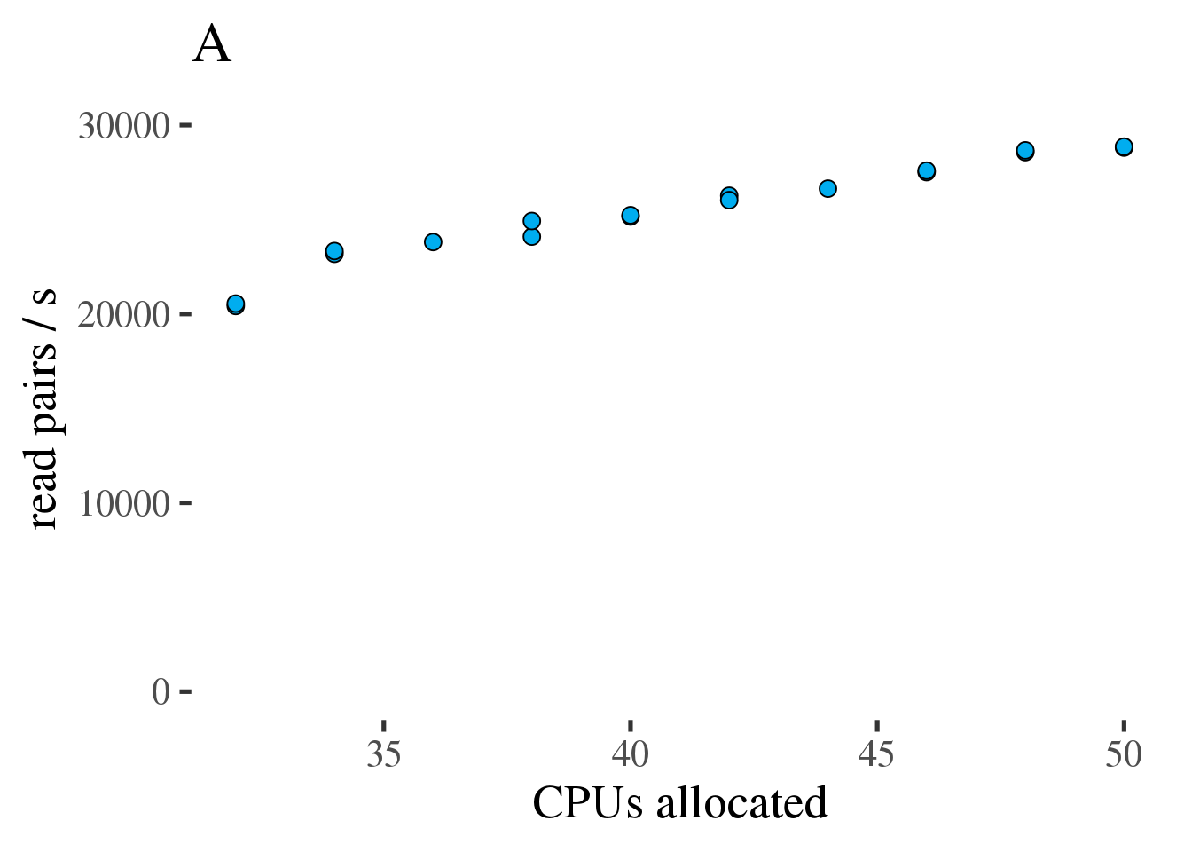
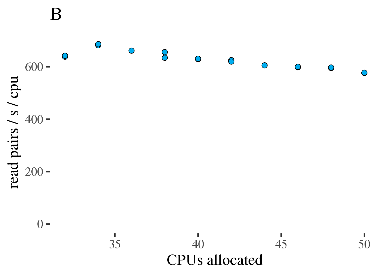
(A) Gross throughput in reads/s of the combined preprocessing pipeline from FASTQ to alignments in a BAM file. The total thread count across all three tools. (B) Like the plot on the left but showing Reads/s/cpu, a measure of efficiency.

Figure 1.7: (A) Gross throughput in reads/s of the combined preprocessing pipeline from FASTQ to alignments in a BAM file. The total thread count across all three tools. (B) Like the plot on the left but showing Reads/s/cpu, a measure of efficiency.

Based on this test we conclude that running the combined preprocessing steps with 50 threads on 34 CPUs is the most efficient approach.

1.5 Read groups

The SAM format specification uses read groups (the @RG header) to associate reads with with different sources (flowcells, lanes, libraries, etc.). Downstream tools use this information as co-variates when modeling errors. However, read groups is used slightly differently by different tools. See how GATK and sentieon recommend using read groups.

In this example there are 4 lanes of HiSeq 2000 data for each sample spread across a number of flow cells. The unique read group id for each lane is sample.flowcell.lane.acc.

1.6 Processing the example trio

Example scripts that implement the optimized approaches from both alternatives described above is available for download here.

The 4 lanes of sequencing data for each of the three samples in our example trio can be trimmed, aligned, and sorted as shown below.

tar -xzf trio_tutoria.tgz
module load jq
cd trio_tutorial/01-preproc
for sample in NA12878 NA12891 NA12892 ; do
    [[ -e ${sample}.json ]] || ./mkconfig $sample | jq '.' > ${sample}.json
done

### check out the created config files
### then submit jobs

mkdir -p data
for sample in NA12878 NA12891 NA12892 ; do
    # data below are for sorted output. You can choose the unsorted script
    # instead
    sbatch ./01-preproc.sh ${sample}.json \
        /fdb/GATK_resource_bundle/hg38-v0/Homo_sapiens_assembly38.fasta \
        data/${sample}.bam
done

Logfiles, diagnostic files, and sorted BAM files will be saved in ./data/. The jobs were not constrained to a specific node type but some basic stats of the full runs of this Chapter are summarized below (for sorted BAM output):

Sample	Runtime	BAM file size	Mean coverage	CPUh
NA12891	11.5h	115GB	47x	391
NA12892	11.7h	125GB	51x	398
NA12878	11.5h	120GB	47.4x	391

mosdepth is a good tool to look at coverage across all sites:

mkdir -p mosdepth

export MOSDEPTH_Q0=NO_COVERAGE   # 0 -- defined by the arguments to --quantize
export MOSDEPTH_Q1=LOW_COVERAGE  # 1..4
export MOSDEPTH_Q2=CALLABLE      # 5..149
export MOSDEPTH_Q3=HIGH_COVERAGE # 150 ...

module load mosdepth/0.3.0
for sample in NA12891 NA12892 NA12878 ; do
    if [[ -e mosdepth/${sample}.quantized.mosdepth.summary.txt ]] ; then
        printf "skipping %s - already done\n" "$sample"
    else
        mosdepth -t3 -n --quantize 0:1:5:150: mosdepth/$sample.quantized data/$sample.bam
    fi
done

Figure 1.8 (A) shows coverage of all autosomes for the three samples. Figure 1.8 (B) shows coverage of X and Y chromosomes consistent with the expected sex.

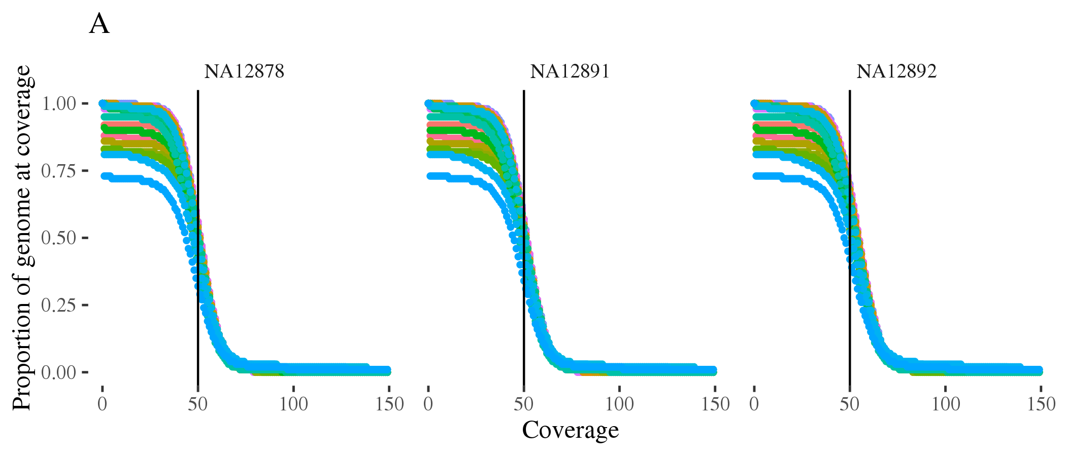
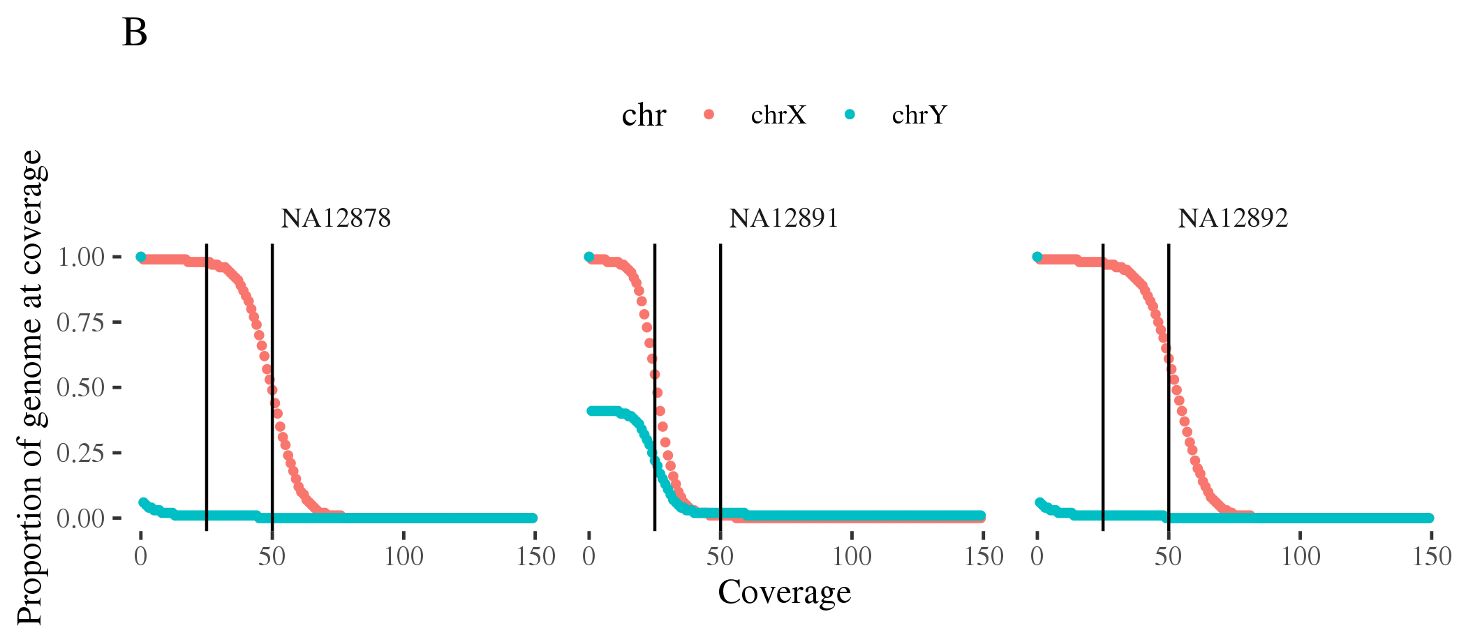
Figure 1.8: Coverage of (A) autosomes and (B) sex chromosomes