The GCN_Cancer application employs graph convolutional network (GCN) models
to classify the gene expression data samples from The Cancer Genonme Atlas (TCAG)
as 33 designated tumor types or as normal. It has been trained on 10,340
cancer samples and 731 normal tissue samples from TCGA dataset.
This application, reimplemented in Keras from the original version developed in Tensorflow,
will be used as a biological example by class #6 of the course
"Deep Learning by Example on Biowulf".
Allocate an interactive session and run the program. Sample session:
[user@biowulf]$ sinteractive  --mem=240g --gres=gpu:a100:1,lscratch:100 -c24
[user@cn4466 ~]$ module load GCN_Cancer
[+] Loading singularity  3.10.3  on cn0830
[+] Loading cuDNN/8.1.0.77/CUDA-11.2.2 libraries...
[+] Loading CUDA Toolkit  11.2.2  ...
[+] Loading GCN_Cancer  20220825
(a lower-case name, gcn_cancer, will also work).
[user@cn4466 ~]$ mkdir -p data
[user@cn4466 ~]$ cp $GCN_CANCER_DATA/{Block_,Adj_}{GCE,GCES,PPI,PPIS}.mat data
Here, the following abbreviations have been used:
GCE  - (gene expression) dataset with gene co-expression type of association between genes
GCES - same as GCE, but additionally includes singleton genes
PPI  - (gene expression) dataset with protein-protein interaction type of association between genes
PPIS - same as PPI, but additionally includes singleton genes
The use of the executable preprocess.py is optional. With proper command line options, it will produce a customized/balanced data matrix and/or a customized adjacency matrix, any or both of which can be (optionally) used as input by the executables train.py and predict.py instead of the original matrices of data samples Block_{GCE,GCES,PPI,PPIS}.mat and/or original adjacency matrices Adj_{GCE,PPI}.mat. that are provided together with the GCN_Cancer code.
user@cn4466 ~]$ preprocess.py -h
usage: preprocess.py [-h] [-A] [-B] [-d data_type] [-f fold] [-N num_elements]
                     [-S smote_variant] [-t threshold] [-v]

optional arguments:
  -h, --help            show this help message and exit
  -A, --custom_adjacency
                        compute the custom adjacency matrix
  -B, --balance_data    balance training data
  -f fold, --fold fold  id of the portion of input data to be used for prediction:
                        0 | 1 | 2 | 3 | 4; default=4
  -N num_elements, --num_elements num_elements
                        target number of nonzero elements in a custom
                        adjacency matrix
  -S smote_variant, --smote_variant smote_variant
                        smote alrorithm to be used for data balancing: SMOTE |
                        SMOTE_TomekLinks | SMOTE_ENN | Borderline_SMOTE1 |
                        Borderline_SMOTE1 | Borderline_SMOTE2 | ADASYN | AHC |
                        LLE_SMOTE | distance_SMOTE | SMMO | polynom_fit_SMOTE
                        | Stefanowski | ADOMS | Safe_Level_SMOTE | MSMOTE |
                        DE_oversampling | SMOBD | SUNDO | MSYN | SVM_balance |
                        TRIM_SMOTE | SMOTE_RSB | ProWSyn | SL_graph_SMOTE |
                        NRSBoundary_SMOTE | LVQ_SMOTE | SOI_CJ | ROSE |
                        SMOTE_OUT | SMOTE_Cosine | Selected_SMOTE | LN_SMOTE |
                        MWMOTE | PDFOS | IPADE_ID | RWO_sampling | NEATER |
                        DEAGO | Gazzah | MCT | ADG | SMOTE_IPF | KernelADASYN
                        | MOT2LD | V_SYNTH | OUPS | SMOTE_D | SMOTE_PSO |
                        CURE_SMOTE | SOMO | ISOMAP_Hybrid | CE_SMOTE |
                        Edge_Det_SMOTE | CBSO | E_SMOTE | DBSMOTE | ASMOBD |
                        Assembled_SMOTE | SDSMOTE | DSMOTE | G_SMOTE |
                        NT_SMOTE | Lee | SPY | SMOTE_PSOBAT | MDO |
                        Random_SMOTE | ISMOTE | VIS_RST | GASMOTE | A_SUWO |
                        SMOTE_FRST_2T | AND_SMOTE | NRAS | AMSCO | SSO |
                        NDO_sampling | DSRBF | Gaussian_SMOTE | kmeans_SMOTE |
                        Supervised_SMOTE | SN_SMOTE | CCR | ANS |
                        cluster_SMOTE | SYMPROD
  -t threshold, --threshold threshold
                        threshold to be used when generating adjacency matrix;
                        default=None
  -v, --verbose         increase the verbosity level of output

required arguments:
  -d data_type, --data_type data_type
                        data type: gce | gces | ppi | ppis
For example, in order to generate a custom data matrix Block_GCE.B.mat balanced using the naive balancing algoritm, run the command:
[user@cn4466 ~]$ preprocess.py -d gce -BIn order to generate a custom data matrix balanced using one of the SMOTE variant algorithms, additionally pass the name of that algorith with option -S. We recommend using either MWMOTE or LLE_SMOTE algorithm. For example, in order to produce the custom data matrix Block_GCE.B.S_MWMOTE.mat, which is balanced using the SMOTE variant algorithm MWMOTE, run the command:
[user@cn4466 ~]$ preprocess.py -d gce -B -S MWMOTETo generate a custom adjacency matrix, specify the option -A and either the target threshold or target number of nonzero elements in the adjacency matrix. For example:
[user@cn4466 ~]$ preprocess.py -d gce -A -t 0.7
...
[user@cn4466 ~]$ preprocess.py -d gce -A -N 10000
...
The usage of the training executable train.py is as follows:
[user@cn4466 ~]$ train.py -h
usage: train.py [-h] [-A] [-b batch_size] [-B] [-d data_type]
                [-D dropout_fraction] [--debug DEBUG] [-f fold] [-g num_gpus]
                [-i input_checkpoint_file] [-I initializer] [-k num_kernels]
                [-l learning_rate] [-L num_levels] [-e num_epochs] [-K K]
                [-m model_name] [-N num_elements] [-O optimizer]
                [-p pooling_layer] [-r ratio] [-S smote_variant]
                [-t threshold] [-v] [-w]

optional arguments:
  -h, --help            show this help message and exit
  -A, --custom_adjacency
                        use custom adjacency matrix
  -b batch_size, --bs batch_size
                        batch size; default=50
  -B, --use_balanced_data
                        use balanced data
  -D dropout_fraction, --dropout_fraction dropout_fraction
                        dropout_fraction; default = 0.0
  --debug DEBUG         use a small subset of data for training
  -f fold, --fold fold  -f fold, --fold fold  id of the portion of input data to be used for prediction:
                        0 | 1 | 2 | 3 | 4; default=4
  -g num_gpus, --num_gpus num_gpus
                        number of gpus to use; default=1
  -i input_checkpoint_file, --input_checkpoint_file input_checkpoint_file
                        input checkpoint file name; default: None
  -I initializer, --initializer initializer
                        Keras weight initializer: glorot_uniform |
                        glorot_normal | he_uniform | he_normal |
                        truncated_unifirmn | truncated_normal| random_unifoirm
                        | random_normal | constant | zeros | ones | orthogonal
                        | variance_scaling ; default = glorot_uniform
  -k num_kernels, --num_kernels num_kernels
                        num. of kernals to be used by Graph Conv layer;
                        default=64
  -l learning_rate, --lr learning_rate
                        learning rate; default=1.e-4
  -L num_levels, --num_levels num_levels
                        # of in the gc/pooling levels in the model: >= 1;
                        default=1
  -e num_epochs, --num_epochs num_epochs
                        num # of epochs; default=10
  -K K                  The hyperparameter K in ChebConv layer; default=1
  -m model_name, --model_name model_name
                        model name: chebnet | gcnnet | densenet | gatnet;
                        default = chebnet
  -N num_elements, --num_elements num_elements
                        target number of nonzero elements in a custom
                        adjacency matrix
  -O optimizer, --optimizer optimizer
                        optimizer: adam | rmsprop
  -p pooling_layer, --pooling_layer pooling_layer
                        pooling layer: DiffPool | MinCutPool; default=DiffPool
  -r ratio, --ratio ratio
                        pooling ratio; default=1.0
  -S smote_variant, --smote_variant smote_variant
                        smote alrorithm: OUPS | SMOTE_D | NT_SMOTE | Gazzah |
                        ROSE; default = OUPS
  -t threshold, --threshold threshold
                        threshold to be used when generating adjacency matrix;
                        default=None
  -v, --verbose         increase the verbosity level of output
  -w, --load_weights    read weights from a checkpoint file

required arguments:
  -d data_type, --data_type data_type
                        data type: gce | gces | ppi | ppis
For example, the simplest command to train the (default) model chebnet on the original data GCE would be:
[user@cn4466 ~]$ train.py -d gce
...
Epoch 1/50
74/74 [==============================] - 103s 1s/step - loss: 1.7426
Epoch 2/50
74/74 [==============================] - 102s 1s/step - loss: 0.6460
Epoch 3/50
74/74 [==============================] - 102s 1s/step - loss: 0.4303
Epoch 4/50
74/74 [==============================] - 102s 1s/step - loss: 0.3378
Epoch 5/50
74/74 [==============================] - 102s 1s/step - loss: 0.2936
Epoch 6/50
74/74 [==============================] - 102s 1s/step - loss: 0.2584
...
...
The result of the training (i.e. network weights) will be stored in the checkpoint file located in the folder "checkpoints", in this particular case, the file
checkpoints/chebnet.gce.D_0.1.h5(here, 0.1 is the default dropout rate used by the models) To train another model on the same data, specify the model name with command line option -m
[user@cn4466 ~]$ train.py -d gce -m gcnnet
...
whcich will produce a checkpoint file checkpoints/gcnnet.gce.D_0.1.h5 In order to train a model on custom data generated by the executable preprocess.py, use additionally the options that match the options used by that executable. For example:
[user@cn4466 ~]$ train.py -d gce -B -S MWMOTE -A -t 0.7
...
[user@cn4466 ~]$ train.py -d gce -B -S MWMOTE -A -N 10000
The command line options for the executable predict.py are similar to, and shoulkd be consistent with, the options that were used by the training command:
[user@cn4466 ~]$ predict.py -h
[user@cn4338 6_GCNs]$ predict.py -h
usage: predict.py [-h] [-A] [-b batch_size] [-B] [-d data_type]
                  [-D dropout_fraction] [--debug DEBUG] [-f fold]
                  [-g num_gpus] [-i input_checkpoint_file] [-I initializer]
                  [-k num_kernels] [-l learning_rate] [-L num_levels]
                  [-e num_epochs] [-K K] [-m model_name] [-N num_elements]
                  [-O optimizer] [-p pooling_layer] [-r ratio]
                  [-S smote_variant] [-t threshold] [-v] [-w]

optional arguments:
  -h, --help            show this help message and exit
  -A, --custom_adjacency
                        use custom adjacency matrix
  -b batch_size, --bs batch_size
                        batch size; default=50
  -B, --use_balanced_data
                        use balanced data
  -D dropout_fraction, --dropout_fraction dropout_fraction
                        dropout_fraction; default = 0.0
  --debug DEBUG         use a small subset of data for training
  -f fold, --fold fold  id of the input data subset to be used for prediction:
                        0 | 1| 2 | 3 | 4; default=4
  -g num_gpus, --num_gpus num_gpus
                        number of gpus to use; default=1
  -i input_checkpoint_file, --input_checkpoint_file input_checkpoint_file
                        input checkpoint file name; default: None
  -I initializer, --initializer initializer
                        Keras weight initializer: glorot_uniform |
                        glorot_normal | he_uniform | he_normal |
                        truncated_unifirmn | truncated_normal| random_unifoirm
                        | random_normal | constant | zeros | ones | orthogonal
                        | variance_scaling ; default = glorot_uniform
  -k num_kernels, --num_kernels num_kernels
                        num. of kernals to be used by Graph Conv layer;
                        default=64
  -l learning_rate, --lr learning_rate
                        learning rate; default=1.e-4
  -L num_levels, --num_levels num_levels
                        # of in the gc/pooling levels in the model: >= 1;
                        default=1
  -e num_epochs, --num_epochs num_epochs
                        num # of epochs; default=10
  -K K                  The hyperparameter K in ChebConv layer; default=1
  -m model_name, --model_name model_name
                        model name: chebnet | gcnnet | densenet | gatnet;
                        default = chebnet
  -N num_elements, --num_elements num_elements
                        target number of nonzero elements in a custom
                        adjacency matrix
  -O optimizer, --optimizer optimizer
                        optimizer: adam | rmsprop
  -p pooling_layer, --pooling_layer pooling_layer
                        pooling layer: DiffPool | MinCutPool; default=DiffPool
  -r ratio, --ratio ratio
                        pooling ratio; default=1.0
  -S smote_variant, --smote_variant smote_variant
                        smote alrorithm: OUPS | SMOTE_D | NT_SMOTE | Gazzah |
                        ROSE; default = OUPS
  -t threshold, --threshold threshold
                        threshold to be used when generating adjacency matrix;
                        default=0.6
  -v, --verbose         increase the verbosity level of output
  -w, --load_weights    read weights from a checkpoint file

required arguments:
  -d data_type, --data_type data_type
                        data type: gce | gces | ppi | ppis
For example, the command
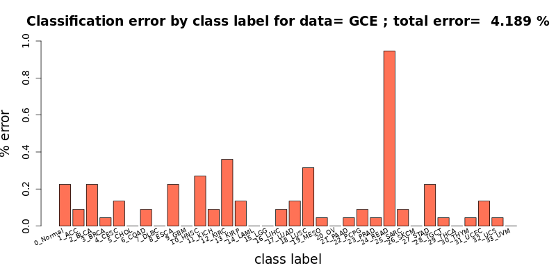
[user@cn4466 ~]$ predict.py -d gce -D 0.1
...
will use pre-trained weights stored in the checkpoint file checkpoints/chebnet.gce.D_0.1.h5 to make predictions of the class labels for the "testing" portion of the input data file Block_GCE.matR. By default, the last of the five available data portions ("folds") will be used for testing/prediction, while the ramining four portions - for training the model. The predict.py command shown above will output the results file results/chebnet.gce.D_0.1.tsv. In order to use a different way of splitting of the input data into the training and testing dataset, specify the id of the portion/fold of the data to be used for prediction, with option -f.
[user@cn4466 ~]$ cat results/chebnet.gce.D_0.1.tsv
#class incorr  total    %err    type
0       5       146     3.425   0_Normal
1       2       19      10.526  1_ACC
2       5       84      5.952   2_BLCA
3       1       226     0.442   3_BRCA
4       3       67      4.478   4_CESC
5       0       5       0.000   5_CHOL
6       2       77      2.597   6_COAD
7       0       7       0.000   7_DLBC
8       5       30      16.667  8_ESCA
9       0       33      0.000   9_GBM
10      6       92      6.522   10_HNSC
11      2       12      16.667  11_KICH
12      8       115     6.957   12_KIRC
13      3       51      5.882   13_KIRP
14      0       43      0.000   14_LAML
15      0       107     0.000   15_LGG
16      2       76      2.632   16_LIHC
17      3       109     2.752   17_LUAD
18      7       103     6.796   18_LUSC
19      1       25      4.000   19_MESO
20      0       83      0.000   20_OV
21      1       23      4.348   21_PAAD
22      2       46      4.348   22_PCPG
23      1       86      1.163   23_PRAD
24      21      36      58.333  24_READ
25      2       44      4.545   25_SARC
26      0       93      0.000   26_SKCM
27      5       78      6.410   27_STAD
28      1       18      5.556   28_TGCT
29      0       109     0.000   29_THCA
30      1       20      5.000   30_THYM
31      3       122     2.459   31_UCEC
32      1       14      7.143   32_UCS
33      0       21      0.000   33_UVM


# Finally: num_corr=2127 / 2220, error= 4.189189 %
#
# 0_Normal -> 2_BLCA: 1 (0.045045 %)
# 0_Normal -> 12_KIRC: 1 (0.045045 %)
# 0_Normal -> 15_LGG: 1 (0.045045 %)
# 0_Normal -> 23_PRAD: 1 (0.045045 %)
# 0_Normal -> 27_STAD: 1 (0.045045 %)
# 1_ACC -> 2_BLCA: 2 (0.090090 %)
# 2_BLCA -> 4_CESC: 3 (0.135135 %)
# 2_BLCA -> 10_HNSC: 1 (0.045045 %)
# 2_BLCA -> 18_LUSC: 1 (0.045045 %)
# 3_BRCA -> 0_Normal: 1 (0.045045 %)
# 4_CESC -> 6_COAD: 1 (0.045045 %)
# 4_CESC -> 31_UCEC: 2 (0.090090 %)
# 6_COAD -> 24_READ: 2 (0.090090 %)
# 8_ESCA -> 27_STAD: 5 (0.225225 %)
# 10_HNSC -> 0_Normal: 1 (0.045045 %)
# 10_HNSC -> 4_CESC: 3 (0.135135 %)
# 10_HNSC -> 18_LUSC: 1 (0.045045 %)
# 10_HNSC -> 25_SARC: 1 (0.045045 %)
# 11_KICH -> 12_KIRC: 1 (0.045045 %)
# 11_KICH -> 13_KIRP: 1 (0.045045 %)
# 12_KIRC -> 0_Normal: 1 (0.045045 %)
# 12_KIRC -> 2_BLCA: 1 (0.045045 %)
# 12_KIRC -> 11_KICH: 1 (0.045045 %)
# 12_KIRC -> 13_KIRP: 3 (0.135135 %)
# 12_KIRC -> 16_LIHC: 1 (0.045045 %)
# 12_KIRC -> 25_SARC: 1 (0.045045 %)
# 13_KIRP -> 2_BLCA: 2 (0.090090 %)
# 13_KIRP -> 12_KIRC: 1 (0.045045 %)
# 16_LIHC -> 0_Normal: 1 (0.045045 %)
# 16_LIHC -> 5_CHOL: 1 (0.045045 %)
# 17_LUAD -> 18_LUSC: 2 (0.090090 %)
# 17_LUAD -> 31_UCEC: 1 (0.045045 %)
# 18_LUSC -> 2_BLCA: 1 (0.045045 %)
# 18_LUSC -> 10_HNSC: 2 (0.090090 %)
# 18_LUSC -> 17_LUAD: 3 (0.135135 %)
# 18_LUSC -> 21_PAAD: 1 (0.045045 %)
# 19_MESO -> 25_SARC: 1 (0.045045 %)
# 21_PAAD -> 25_SARC: 1 (0.045045 %)
# 22_PCPG -> 0_Normal: 1 (0.045045 %)
# 22_PCPG -> 21_PAAD: 1 (0.045045 %)
# 23_PRAD -> 0_Normal: 1 (0.045045 %)
# 24_READ -> 6_COAD: 21 (0.945946 %)
# 25_SARC -> 16_LIHC: 1 (0.045045 %)
# 25_SARC -> 32_UCS: 1 (0.045045 %)
# 27_STAD -> 8_ESCA: 4 (0.180180 %)
# 27_STAD -> 28_TGCT: 1 (0.045045 %)
# 28_TGCT -> 29_THCA: 1 (0.045045 %)
# 30_THYM -> 10_HNSC: 1 (0.045045 %)
# 31_UCEC -> 12_KIRC: 1 (0.045045 %)
# 31_UCEC -> 20_OV: 1 (0.045045 %)
# 31_UCEC -> 32_UCS: 1 (0.045045 %)
# 32_UCS -> 31_UCEC: 1 (0.045045 %)
# 33_UVM -> 26_SKCM: 1 (0.045998 %)
Here, the label 0 corresponds to the Normal samples, and the following abbreviations have been used to designate the 33 tumor types, with labels 1 to 33:
ACC     Adrenocortical carcinoma
BLCA    Bladder Urothelial Carcinoma
BRCA    Breast invasive carcinoma
CESC    Cervical squamous cell carcinoma and endocervical adenocarcinoma
CHOL    Cholangiocarcinoma
COAD    Colon adenocarcinoma
DLBC    Lymphoid Neoplasm Diffuse Large B-cell Lymphoma
ESCA    Esophageal carcinoma
GBM     Glioblastoma multiforme
HNSC    Head and Neck squamous cell carcinoma
KICH    Kidney Chromophobe
KIRC    Kidney renal clear cell carcinoma
KIRP    Kidney renal papillary cell carcinoma
LAML    Acute Myeloid Leukemia
LGG     Brain Lower Grade Glioma
LIHC    Liver hepatocellular carcinoma
LUAD    Lung adenocarcinoma
LUSC    Lung squamous cell carcinoma
MESO    Mesothelioma
OV      Ovarian serous cystadenocarcinoma
PAAD    Pancreatic adenocarcinoma
PCPG    Pheochromocytoma and Paraganglioma
PRAD    Prostate adenocarcinoma
READ    Rectum adenocarcinoma
SARC    Sarcoma
SKCM    Skin Cutaneous Melanoma
STAD    Stomach adenocarcinoma
TGCT    Testicular Germ Cell Tumors
THCA    Thyroid carcinoma
THYM    Thymoma
UCEC    Uterine Corpus Endometrial Carcinoma
UCS     Uterine Carcinosarcoma
UVM     Uveal Melanoma
Finally, in order to visualize the summary provided in the results file, run the executable visualize.R:
[user@cn4466 ~]$ visualize.R results/chebnet.gce.D_0.1.tsv
[user@cn4466 ~]$ visualize.R results/chebnet.K_10.gces.D_0.1.B.S_MWMOTE.tsv

[user@cn4466 ~]$ train.py   -d gce -K 20 -B -S MWMOTE -l 1.e-6
[user@cn4466 ~]$ predict.py -d gce -K 20 -B -S MWMOTE
will result in the error-free classification (!).
[user@cn4471 ~]$ exit
[user@biowulf ~] sinteractive --mem=240g --gres=gpu:a100:4,lscratch:100 --cpus-per-task=14
[user@cn4471 ~]$ mkdir -p data
[user@cn4471 ~]$ module load gcn_cancer
[user@cn4471 ~]$ cp $GCN_CANCER_DATA/{Block_,Adj_}{GCE,GCES,PPI,PPIS}.mat data
[user@cn4471 ~]$ train.py -d gces -g 4 -b 2000
End the interactive session:
[user@cn4466 ~]$ exit
salloc.exe: Relinquishing job allocation 46116226
[user@biowulf ~]$
Create a batch input file (e.g. gcn_cancer.sh). For example:
#!/bin/bash
module load GCN_Cancer
mkdir -p data
cp $GCN_CANCER_DATA/{Block_,Adj_}{GCE,GCES,PPI,PPIS}.mat data
train.py  -d gce
Submit this job using the Slurm sbatch command.
sbatch [--cpus-per-task=#] [--mem=#] gcn_cancer.sh