R/Bioconductor on Biowulf

R is a language and environment for statistical computing and graphics. It
can be considered an open source decendant of the S language which was
developed by Chambers and colleagues at Bell Laboratories in the 1970s.
R is highly extensible and provides a wide variety of modern statistical
analysis methods combined with excellent graphical visualization capabilities
embedded in a programming language that supports procedural, functuional, and
object oriented programming styles. R natively provides operators for calculations
on arrays and matrices.
While individual single threaded R code is not expected to run any faster in
an interactive session on a compute node
than it would run on a modern desktop, Biowulf allows users to run many R jobs
concurrently or take advantage of the speedup provided by parallelizing R code
to a much greater degree than possible on a single workstation.
On biowulf, R modules are available for the minor releases (e.g. 4.2) which
will contain the newest patch level releases (e.g. 4.2.3).
- Mar 18, 2026: R/4.5.2 becomes the default R installation.
- Jun 2, 2025: R/4.5.0 becomes the default R installation.
- May 2025: R/4.5.0 is installed, will become the default R installation on June 2nd.
- Mar 10, 2025: R/4.4.3 becomes the default R installation.
- Nov 10, 2024: R/4.4.2 becomes the default R installation.
- Jun 26, 2024: R/4.4.1 becomes the default R installation.
- May 3, 2024: R/4.4.0 becomes the default R installation.
- Jan 2024: R/4.3.2 becomes the default R installation.
- Jun 23 2023: default location for
$R_LIBS_USER
- changed to
/data/$USER/R/rhel8/%v with migration to RHEL8
- May 2023: R/4.3.0 becomes the default R installation.
- User visible changes:
- Calling
&& or || with LHS or (if evaluated)
RHS of length greater than one is now always an error, with a report of the form
'length = 4' in coercion to 'logical(1)'. R 4.2.0 introduced
a warning for this usage of conditional operators.
- Environment variable _R_CHECK_LENGTH_1_LOGIC2_ no longer has any effect.
See R NEWS for
full details.
- Nov 2022: R/4.2.2 becomes the default R installation.
- Jul 2022: R/4.2.0 becomes the default R installation.
- Some notable changes:
- Calling
&& or || with either argument of length greater
than one now gives a warning (which it is intended will become
an error).
- Calling if() or while() with a condition of length greater
than one gives an error rather than a warning. Consequently,
environment variable _R_CHECK_LENGTH_1_CONDITION_ no longer has
any effect.
- The graphics engine version, R_GE_version, has been bumped to 15.
- Jul 2021: R/4.1.0 becomes the default R installation.
- Apr 2021: R/4.0.5 becomes the default R installation. OpenMPI is now version 4
- Nov 2020: R/4.0.3 becomes the default R installation
- Jun 2020: R/4.0.0 becomes the default R installation
- For details see R NEWS. Notable changes:
- R now uses
stringsAsFactors = FALSE as the default
- There is a new syntax for specifying raw character constants similar to the one used in C++: r"(...)"
As usual, many packages are pre-installed and private packages
need to be re-installed.
- Jun 2020: R/4.0.0 becomes the default R installation
- Apr 2020: R/3.6.3 becomes the default R installation
- Dec 2019: R/3.6.1 becomes the default R installation and R is now compiled with gcc 9.2.0
- Jun 2019: R/3.6.0 becomes the default R installation
- Feb 2019: R/3.5.2 becomes the default R installation
- Jun 2018: Cluster update from RHEL6 to RHEL7
-
- R sessions are not allowed on helix any more.
- R is compiled against MKL for improved performance
- Implicit multithreading
-
R can make use of implicit multithreading via two
different mechanisms. One of them is regulated by the
OMP_NUM_THREADS
or MKL_NUM_THREADS
environment variables which are set to 1 by the R wrappers because leaving this
variable unset can lead to R using as many threads as there are CPUs on a compute
node thus overloading jobs. If you know your code can make effective use of those
threads you can explicitly set OMP_NUM_THREADS to greater than 1 after
loading the module. However, only a subset of code will be able to take advantage of
this - don't expect an automatic speed increase.
parallel::detectCores() always detects all CPUs on a node-
R using one of the parallel packages (parallel, doParallel, ...) often overload
their job allocation because they are using the
detectCores() function
from the parallel package to determine how many worker processes to use. However,
this function returns the number of physical CPUs on a compute node irrespective of
how many have been allocated to a job. Therefore, if not all CPUs are allocated to a job
the job will be overloaded and perform poorly. See the section on the
parallel package for more detail.
BiocParallel by default tries to use most CPUs on a node-
BiocParallel is not aware of slurm and by default tries to use most
of the CPUs on a node irrespetive of the slurm allocation. This can lead to overloaded
jobs. See the section on the
BiocParallel package for more information on how to avoid
this.
- Poor scaling of parallel code
-
Don't assume that you should allocate as many CPUs as possible to a parallel workload.
Parallel efficiency often drops and in some cases allocating more CPUs may actually
extend runtimes. If you use/implement parallel algorithms please measure scaling
before submitting large numbers of such jobs.
- Can't install packages in my private library
-
R will attempt to install packages to
/data/R/rhel8/%v (RHEL8) where %v is the two
digit version of R (e.g. 4.1) or in the path set by $R_LIBS_USER.
However, R won't always automatically create that directory and in
its absence will try to install to the central packge library which will fail. If you encounter
installation failures please make sure the library directory for your version of R exists.
- AnnotationHub or ExperimentHub error
No internet connection
-
The AnnotationHub and ExperimentHub packages and packages depending on them need to connect to the
internet via a proxy. When using AnnotationHub or ExperimentHub directly, a proxy can be specified
explicitly in the call to set up the Hub. However, if they are used indirectly that is not possible.
Instead, define the proxy either using environment variables EXPERIMENT_HUB_PROXY/ANNOTATION_HUB_PROXY
or by setting options in R with
setAnnotationHubOption("PROXY", Sys.getenv("http_proxy"))
or the corresponding setExperimentHubOption function.
- Updating broken packages installed in home directory
-
When R and/or the centrally installed R packages are updated, packages installed in your
private library may break or result in other packages not loading. The most common error
results from a locally installed
rlang package. Look for errors that
include your private library path in the errors. All locally
installed package can be updated with
> my.lib <- .libPaths()[1]  # check first that .libPaths()[1] is indeed the path to your library
> my.pkgs <- list.files(my.lib)
> library(pacman)
> p_install(pkgs, character.only=T, lib=my.lib)
An easy way to fix this error is also to delete the locally installed rlang with
$ rm -rf ~/R/4.2/library/rlang # replace 4.2 with the R major.minor version you are using
- Re-install packages to 1) data directory from home directory and/or 2) different R version
-
Since R_LIBS_USER was relocated to data directory, the R packages installed in your
private library (at ~/R/) need to be reinstalled. And/or if you need to update to a newer R version by reinstalling
all the packages from an older version of R. Let's create the private library directory for the new version of R first (e.g. R/4.5):
$ mkdir -p /data/$USER/R/rhel8/4.5/
For example, for packages installed under R/4.4, you can re-install them by creating a list of installed libraries, find
the ones that are not yet installed under data directory or not the same R version you are using, then re-install them with:
# Get the list of installed packages in R version 4.4 using the current user's directory
packages <- installed.packages(lib.loc=paste0("/data/", Sys.getenv("USER"), "/R/rhel8/4.4"))[,"Package"]

# Identify packages that are not installed in R version 4.5
toInstall <- setdiff(packages, installed.packages(loc.lib=paste0("/data/", Sys.getenv("USER"), "/R/rhel8/4.5/"))[,"Package"])

# Install the missing packages using BiocManager
BiocManager::install(toInstall)
R will automatically use lscratch
for temporary files if it has been allocated. Therefore we highly recommend users always
allocate a minimal amount of lscratch of 1GB plus whatever lscratch storage is required by
your code.
Allocate an interactive session for
interactive R work. Note that R sessions are not allowed on the login node
nor helix.
[user@biowulf]$ sinteractive --gres=lscratch:5
salloc.exe: Pending job allocation 46116226
salloc.exe: job 46116226 queued and waiting for resources
salloc.exe: job 46116226 has been allocated resources
salloc.exe: Granted job allocation 46116226
salloc.exe: Waiting for resource configuration
salloc.exe: Nodes cn3144 are ready for job
There may be multiple versions of R available. An easy way of selecting the
version is to use modules.To see the modules
available, type
[user@cn3144 ~]$ module -r avail '^R$'

--------------- /usr/local/lmod/modulefiles ------------------
R/3.4    R/3.4.3    R/3.4.4    R/3.5 (D)    R/3.5.0    R/3.5.2
Set up your environment and start up an R session
[user@cn3144 ~]$ module load R/3.5
[user@cn3144 ~]$ R
R version 3.5.0 (2018-04-23) -- "Joy in Playing"
Copyright (C) 2018 The R Foundation for Statistical Computing
Platform: x86_64-pc-linux-gnu (64-bit)

R is free software and comes with ABSOLUTELY NO WARRANTY.
You are welcome to redistribute it under certain conditions.
Type 'license()' or 'licence()' for distribution details.

  Natural language support but running in an English locale

R is a collaborative project with many contributors.
Type 'contributors()' for more information and
'citation()' on how to cite R or R packages in publications.

Type 'demo()' for some demos, 'help()' for on-line help, or
'help.start()' for an HTML browser interface to help.
Type 'q()' to quit R.

> library(tidyverse)
── Attaching packages ─────────────────────────────────────── tidyverse 1.2.1 ──
✔ ggplot2 2.2.1     ✔ purrr   0.2.4
✔ tibble  1.4.2     ✔ dplyr   0.7.4
✔ tidyr   0.8.0     ✔ stringr 1.3.0
✔ readr   1.1.1     ✔ forcats 0.3.0
── Conflicts ────────────────────────────────────────── tidyverse_conflicts() ──
✖ dplyr::filter() masks stats::filter()
✖ dplyr::lag()    masks stats::lag()
> [...lots of work...]
> q()
Save workspace image? [y/n/c]: n
A rudimentary graphical interface is available if the sinteractive
session was started from a session with X11 forwarding enabled:
[user@cn3144 ~]$ R --gui=Tk
However, RStudio is a much better interface
with many advanced features.
Don't forget to exit the interactive session
[user@cn3144 ~]$ exit
salloc.exe: Relinquishing job allocation 46116226
[user@biowulf ~]$
Per-user R library
Users can install their own packages. By default, on RHEL8, this private library
is located at /data/$USER/R/rhel8/%v where %v
is the major.minor version of R (e.g. 4.3). This is a change from the
behaviour on RHEL7 where the default location was ~/R/%v/library.
Note that this directory is not created automatically by some
versions of R so it is safest to create it manually before installing R
packages.
Users can choose alternative locations for this directory by setting and
exporting the environment variable $R_LIBS_USER in your shell
startup script. If you are a bash user, for example, you could add the
following line to your ~/.bash_profile to relocated your R
library:
export R_LIBS_USER="/data/$USER/code/R/rhel8/%v"
Here is an example using the pacman
package for easier package management:
[user@cn3144 ~]$ R

R version 4.1.0 (2021-05-18) -- "Camp Pontanezen"
Copyright (C) 2021 The R Foundation for Statistical Computing
Platform: x86_64-pc-linux-gnu (64-bit)

> library(pacman)
> p_isinstalled(rapport)
[1] FALSE
> p_install(rapport)
Installing package into ‘/spin1/home/linux/user/R/4.1/library’
(as ‘lib’ is unspecified)
also installing the dependency ‘rapportools’

trying URL 'http://cran.rstudio.com/src/contrib/rapportools_1.0.tar.gz'

[...snip...]
rapport installed
>
More granular (and reproducible) package management
A better approach than relying on packages installed centrally or in
your home directory is to create isolated, per project package sets. This
increases reproducibility at the cost of increased storage and potential
package installation headaches. Some packages to implement this:
- Recommended: The renv package
is a more modern replacement for packrat.
- The older packrat package implements isolated per
project R libraries. See the packrat walkthrough
for a basic introduction.
R batch jobs are similar to any other batch job. A batch script ('rjob.sh')
is created that sets up the environment and runs the R code:
#!/bin/bash

module load R/4.2
R --no-echo --no-restore --no-save < /data/user/Rtests/Rtest.r > /data/user/Rtests/Rtest.out
or use Rscript instead
#!/bin/bash

module load R/3.5
Rscript /data/user/Rtests/Rtest.r > /data/user/Rtests/Rtest.out
Submit this job using the Slurm sbatch command.
sbatch [--cpus-per-task=#] [--mem=#] rjob.sh
Command line arguments for R scripts
R scripts can be written to accept command line arguments. The simplest
way of doing this is with the commandArgs() function. For
example the script 'simple_args.R'
args <- commandArgs(trailingOnly=TRUE)

i <- 0
for (arg in args) {
    i <- i + 1
    cat(sprintf("arg %02i: '%s'\n", i, arg))
}
can be called like this
[user@cn3144]$ module load R
[user@cn3144]$ Rscript simple.R this is a test
arg 01: 'this'
arg 02: 'is'
arg 03: 'a'
arg 04: 'test'
[user@cn3144]$ Rscript simple.R 'this is a test'
arg 01: 'this is a test'
[user@cn3144]$ R --no-echo --no-restore --no-save --args 'this is a test' < simple.R
arg 01: 'this is a test'
Alternatively, commandline arguments can be parsed using the getopt package. For example:
library(getopt)

###
### Describe the expected command line arguments
###
# mask: 0=no argument
#       1=required argument
#       2=optional argument
spec <- matrix(c(
# long name  short name  mask  type          description(optional)
# ---------  ----------  ----  ------------  ---------------------
  'file'   , 'f',          1,  'character',  'input file',
  'verbose', 'v',          0,  'logical',    'verbose output',
  'help'   , 'h',          0,  'logical',    'show this help message'
), byrow=TRUE, ncol=5);

# parse the command line
opt <- getopt(spec);

# show help if requested
if (!is.null(opt$help)) {
  cat(getopt(spec, usage=TRUE));
  q();
}

# set defaults
if ( is.null(opt$file) )    { opt$file    = 'testfile' }
if ( is.null(opt$verbose) ) { opt$verbose = FALSE }
print(opt)
This script an be used as follows
[user@cn3144]$ Rscript getopt_example.R --file some.txt --verbose
$ARGS
character(0)

$file
[1] "some.txt"

$verbose
[1] TRUE

[user@cn3144]$ Rscript getopt_example.R --file some.txt
$ARGS
character(0)

$file
[1] "some.txt"

$verbose
[1] FALSE

[user@cn3144]$ Rscript getopt_example.R --help
Usage: getopt_example.R [-[-file|f] ] [-[-verbose|v]] [-[-help|h]]
    -f|--file       input file
    -v|--verbose    verbose output
    -h|--help       show this help message
getopt does not have support for mixing flags and positional arguments.
There are other packages with different features and approaches that can
be used to design command line interfaces for R scripts.
A swarm of jobs is an easy way to submit a
set of independent commands requiring identical resources.
Create a swarmfile (e.g. rjobs.swarm). For example:
Rscript /data/user/R/R1  > /data/user/R/R1.out
Rscript /data/user/R/R2  > /data/user/R/R2.out
Rscript /data/user/R/R3  > /data/user/R/R3.out
Submit this job using the swarm command.
swarm -f TEMPLATE.swarm [-g #] [-t #] --module R/3.5
where
| -g # | Number of Gigabytes of memory required for each process (1 line in the swarm command file)
|
| -t # | Number of threads/CPUs required for each process (1 line in the swarm command file).
|
| --module TEMPLATE | Loads the TEMPLATE module for each subjob in the swarm
|
Rswarm is a utility to create a series of R input files from a
single R (master) template file with different output filenames and with unique
random number generator seeds. It will simultaneously create a swarm command
file that can be used to submit the swarm of R jobs. Rswarm was originally
developed by Lori Dodd and Trevor Reeve with modifications by the Biowulf
staff.
Say, for example, that the goal of a simulation study is to evaluate
properties of the t-test. The function "sim.fun" in file "sim.R" below
repeatedly generates random normal data with a given mean, performs a one
sample t-test (i.e. testing if the mean is different from 0), and records the
p-values.
#######################################
# n.samp:  size of samples generated for each simulation
# mu:      mean
# sd:      standard deviation
# nsim:    the number of simulations
# output1: output table
# seed:    the seed for set.seed
#######################################
sim.fun <- function(n.samp=100, mu=0, sd=1, n.sim, output1, seed){

    set.seed(seed)

    p.values <- c()
    for (i in 1:n.sim){
        x <- rnorm(n.samp, mean=mu, sd=sd)
        p.values <- c(p.values, t.test(x)$p.value)
    }
    saveRDS(p.values, file=output1)
}
To use Rswarm, create a wrapper script similar to the following ("rfile.R")
source("sim.R")
sim.fun(n.sim=DUMX, output1="DUMY1",seed=DUMZ)
using the the dummy variables which will be replaced by Rswarm.
| Dummy variable | Replaced with |
|---|
| DUMX | Number of simulations to be specified in each replicate file |
| DUMY1 | Output file 1 |
| DUMY2 | Output file 2 (optional) |
| DUMZ | Random seed |
To swarm this code, we need replicates of the rfile.R file, each with a
different seed and different output file. The Rswarm utility will create the
specified number of replicates, supply each with a different seed (from an
external file containing seed numbers), and create unique output files for each
replicate. Note, that we allow for you to specify the number of simulations
within each file, in addition to specifying the number of replicates.
For example, the following Rswarm command at the Biowulf prompt will create
2 replicate files, each specifying 50 simulations, a different seed from a
file entitled, "seedfile.txt," and unique output files.
[user@biowulf]$ ls -lh
total 8.0K
-rw-r--r-- 1 user group  63 Apr 25 12:34 rfile.R
-rw-r--r-- 1 user group 564 Apr 25 12:15 seedfile.txt
-rw-r--r-- 1 user group 547 Apr 25 12:04 sim.R
[user@biowulf]$ head -n2 seedfile.txt
24963
27507
[user@biowulf]$ Rswarm --rfile=rfile.R --sfile=seedfile.txt --path=. \
    --reps=2 --sims=50 --start=0 --ext1=.rds
The template file is rfile.R
The seed file is seedfile.txt
The path is .
The number of replicates desired is 2
The number of sims per file is 50
The starting file number is 0+1
The extension for output files 1 is .rds
The extension for output files 2 is .std.txt
Is this correct (y or n)? : y
Creating file number 1: ./rfile1.R with output ./rfile1.rds ./rfile1.std.txt and seed 24963
Creating file number 2: ./rfile2.R with output ./rfile2.rds ./rfile2.std.txt and seed 27507
[user@biowulf]$ ls -lh
total 16K
-rw-r--r-- 1 user group  69 Apr 25 12:39 rfile1.R
-rw-r--r-- 1 user group  69 Apr 25 12:39 rfile2.R
-rw-r--r-- 1 user group  63 Apr 25 12:34 rfile.R
-rw-r--r-- 1 user group  50 Apr 25 12:39 rfile.sw
-rw-r--r-- 1 user group 564 Apr 25 12:15 seedfile.txt
-rw-r--r-- 1 user group 547 Apr 25 12:04 sim.R
[user@biowulf]$ cat rfile1.R
source("sim.R")
sim.fun(n.sim=50, output1="./rfile1.rds",seed=24963)
[user@biowulf]$ cat rfile2.R
source("sim.R")
sim.fun(n.sim=50, output1="./rfile2.rds",seed=27507)
[user@biowulf]$ cat rfile.sw
R --no-echo --no-restore --no-save < ./rfile1.R
R --no-echo --no-restore --no-save < ./rfile2.R
[user@biowulf]$ swarm -f rfile.sw --time=10 --partition=quick --module R
199110
[user@biowulf]$ ls -lh *.rds
-rw-r--r-- 1 user group 445 Apr 25 12:52 rfile1.rds
-rw-r--r-- 1 user group 445 Apr 25 12:52 rfile2.rds
Full Rswarm usage:
Usage: Rswarm [options]
   --rfile=[file]   (required) R program requiring replication
   --sfile=[file]   (required) file with generated seeds, one per line
   --path=[path]    (required) directory for output of all files
   --reps=[i]       (required) number of replicates desired
   --sims=[i]       (required) number of sims per file
   --start=[i]      (required) starting file number
   --ext1=[string]    (optional) file extension for output file 1
   --ext2=[string]    (optional) file extension for output file 2`
   --help, -h         print this help text
Note that R scripts can be written to take a random seed as a command line argument
or derive it from the environment variable SLURM_ARRAY_TASK_ID to achieve
an equivalent result.
Using the parallel package
The R
parallel package provides functions for parallel execution of R code on
machines with multiple CPUs. Unlike other parallel processing methods, all jobs
share the full state of R when spawned, so no data or code needs to be
initialized if it was loaded before starting worker processes. The actual
spawning is very fast as well since no new R instance needs to be started.
Detecting the number of CPUs
Parallel includes the dectectCores function which is often used
to automatically detect the number of available CPUs. However, it always
reports all CPUs available on a node irrespective of how many CPUs
were allocated to the job. This is not the desired behavior for batch jobs
or sinteractive sessions. Instead, please use the availableCores()
function from the future (or parallelly for R >= 4.0.3) package which correctly
returns the number of allocated CPUs:
parallelly::availableCores() # for R >= 4.0.3
# or
future::availableCores()
Or, if you prefer, you could also write your own detection function
similar to the following example
detectBatchCPUs <- function() {
    ncores <- as.integer(Sys.getenv("SLURM_CPUS_PER_TASK"))
    if (is.na(ncores)) {
        ncores <- as.integer(Sys.getenv("SLURM_JOB_CPUS_PER_NODE"))
    }
    if (is.na(ncores)) {
        return(2)
    }
    return(ncores)
}
Random number generation
The state of the random number generator in each worker process has
to be carefully considered for any parallel workloads. See the help for
mcparallel and the parallel package documentation for
more details.
Example 1: mclapply
The mclapply() function calls lapply() in parallel, so that the first two arguments
to mclapply() are exactly the same as for lapply(). Except the mc.cores argument needs
to be specified to split the computatation across multiple CPUs on the same node. In most cases mc.cores
should be equal to the number of allocated CPUs.
> ncpus <- parallelly::availableCores()
> options(mc.cores = ncpus) # set a global option for parallel packages
# Then run mclapply()
> mclapply(X, FUN, ..., mc.cores = ncpus)
Performance comparision between lapply() and mclapply():
> library(parallel)
> ncpus <- parallelly::availableCores()
> N <- 10^6
> system.time(x<-lapply(1:N, function(i) {rnorm(300)}))
##   user  system elapsed
## 36.588   1.375  38.053
> system.time(x<-mclapply(1:N, function(i) {rnorm(300)},mc.cores = ncpus)) #Test on a phase5 node with ncpus=12
##   user  system elapsed
## 11.587  14.547  13.684
In this example, using 12 CPUs with mclapply() only reduced runtime by only 2.8 fold compared to running
on a single CPU. Under ideal conditions, the reduction would have been expected to be 12 fold. This means the work done
per CPU was less in the parallel case than in the sequential (single CPU) case. This is called parallel efficiency.
In this example the efficiency would have been sequential CPU time / parallel CPU time = (38.1 * 1) / (13.7 * 12) = 23%.
Parallel jobs should aim for an efficiency of 70-80%. Because parallel algorithms rarely
scale ideally to multiple CPUs we highly recommend performing scaling test before running programs in parallel.
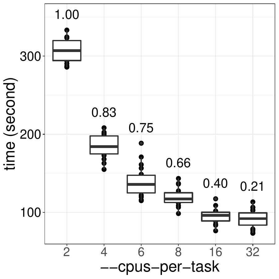
To better optimize the usage of mclapply(), we benchmarked the performance of mclappy() with 2-32 CPUs
and compared their efficiency:
The code used for benchmark was:
> library(parallel)
> library(microbenchmark)
> N <- 10^5
# benchmark the performance with 2-32 CPUs for 20 times
> for (n in c(2,4,6,8,16,32)) {
microbenchmark(mctest = mclapply(1:N, function(i) {rnorm(30000)},mc.cores=n),times = 20)
}
As show in the figure, this particular mclapply() should be run with no more than 6 CPUs
to ensure a higher than 70% of efficiency. This may be different for your code and should be tested
for each type of workload. Note that memory usage increases with more CPUs are used which
makes it even more important to not allocate more CPUs than necessary.
Example 2: foreach
A very convenient way to do parallel computations is provided by the
foreach package. Here
is a simple example (copied from this
blog post)
> library(foreach)
> library(doParallel)
> library(doMC)
> registerDoMC(cores=future::availableCores())
> max.eig <- function(N, sigma) {
     d <- matrix(rnorm(N**2, sd = sigma), nrow = N)
     E <- eigen(d)$values
     abs(E)[[1]] }
> library(rbenchmark)
> benchmark(
     foreach(n = 1:100) %do% max.eig(n, 1),
     foreach(n = 1:100) %dopar% max.eig(n, 1) )

##          test                             replications elapsed relative user.self sys.self user.child sys.child
##1    foreach(n = 1:100) %do% max.eig(n, 1)          100  32.696    3.243 32.632   0.059      0.000      0.00
##2 foreach(n = 1:100) %dopar% max.eig(n, 1)          100  10.083    1.000 3.037    3.389     43.417     10.73
>
Note that with 12 CPUs we got a speedup of only 3.2 relative to sequential
resulting in a low parallel efficiency. Another cautionary tale to
carefully test scaling of parallel code.
A second way to run foreach in parallel:
> library(doParallel)
> cl <- makeCluster(future::availableCores())
> registerDoParallel(cl)
 # parallel command
> ...
 # stop cluster
> stopCluster(cl)
What if we increased the number of tasks and the size of the largest matrix
(i.e. more work per task)? In the example above that means increasing the
i in foreach(n=1:i) using a fixed number of CPUs (32
in this case). We then calculated the speedup relative to execution on 2 CPUs:
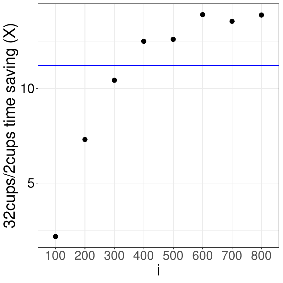
If parallelism was 100% efficient, the speedup would be 16-fold. We recommend
running jobs at 70% parallel efficiency or better which would correspond to a
11-fold speedup in this case (blue horizontal line). In this example, 70% efficiency
is reached at i > 300. That means on biowulf you should only
run this code on 32 CPUs if for i > 300.
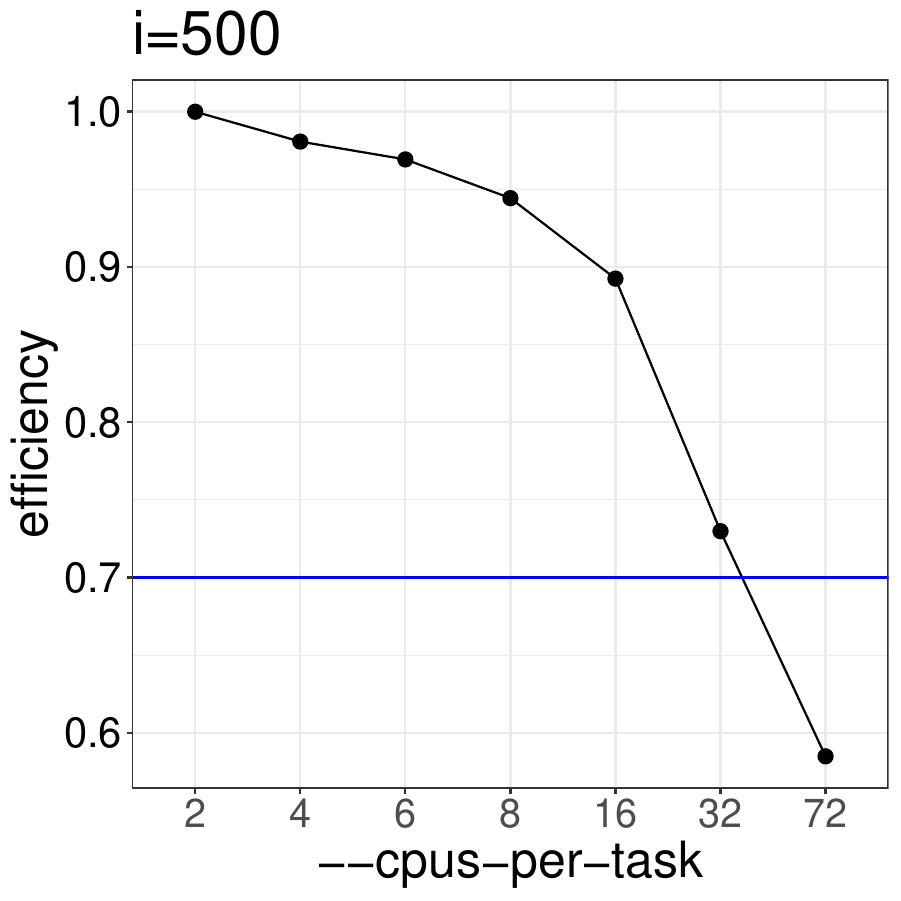
How does the code perform with different numbers of CPUs for i = 500.
Based on the results shown below, this code should be run with no more than 32 CPUs
to ensure that efficiency is better than 70%.
Using the BiocParallel package
The R
BiocParallel provides modified versions and novel implementation of
functions for parallel evaluation, tailored to use with Bioconductor objects. Like
the parallel package, it is not aware of slurm allocations and will therefore,
by default, try to use parallel::detectCores() - 2 CPUs, which is
all but 2 CPUs installed on a compute node irrespective of how many CPUs have
been allocated to a job. That will lead to overloaded jobs and very inefficient
code. You can verify this by checking on the registered backends after allocating
an interactive session with 2 CPUs:
> library(BiocParallel)
> registered()
$MulticoreParam
class: MulticoreParam
  bpisup: FALSE; bpnworkers: 54; bptasks: 0; bpjobname: BPJOB
  bplog: FALSE; bpthreshold: INFO; bpstopOnError: TRUE
  bptimeout: 2592000; bpprogressbar: FALSE
  bpRNGseed:
  bplogdir: NA
  bpresultdir: NA
  cluster type: FORK
[...snip...]
So the default backend (top of the registered stack) would use 54 workers on
2 CPUs. The default backend can be changed with
> options(MulticoreParam=quote(MulticoreParam(workers=future::availableCores())))
> registered()
$MulticoreParam
class: MulticoreParam
  bpisup: FALSE; bpnworkers: 2; bptasks: 0; bpjobname: BPJOB
  bplog: FALSE; bpthreshold: INFO; bpstopOnError: TRUE
[...snip..]
or
> register(MulticoreParam(workers = future::availableCores()), default=TRUE)
Alternatively, a param object can be passed to BiocParallel functions.
R can do implicit multithreading when using a subset of optimized functions
in the library or functions that take advantage of parallelized routines in the
lower level math libraries.
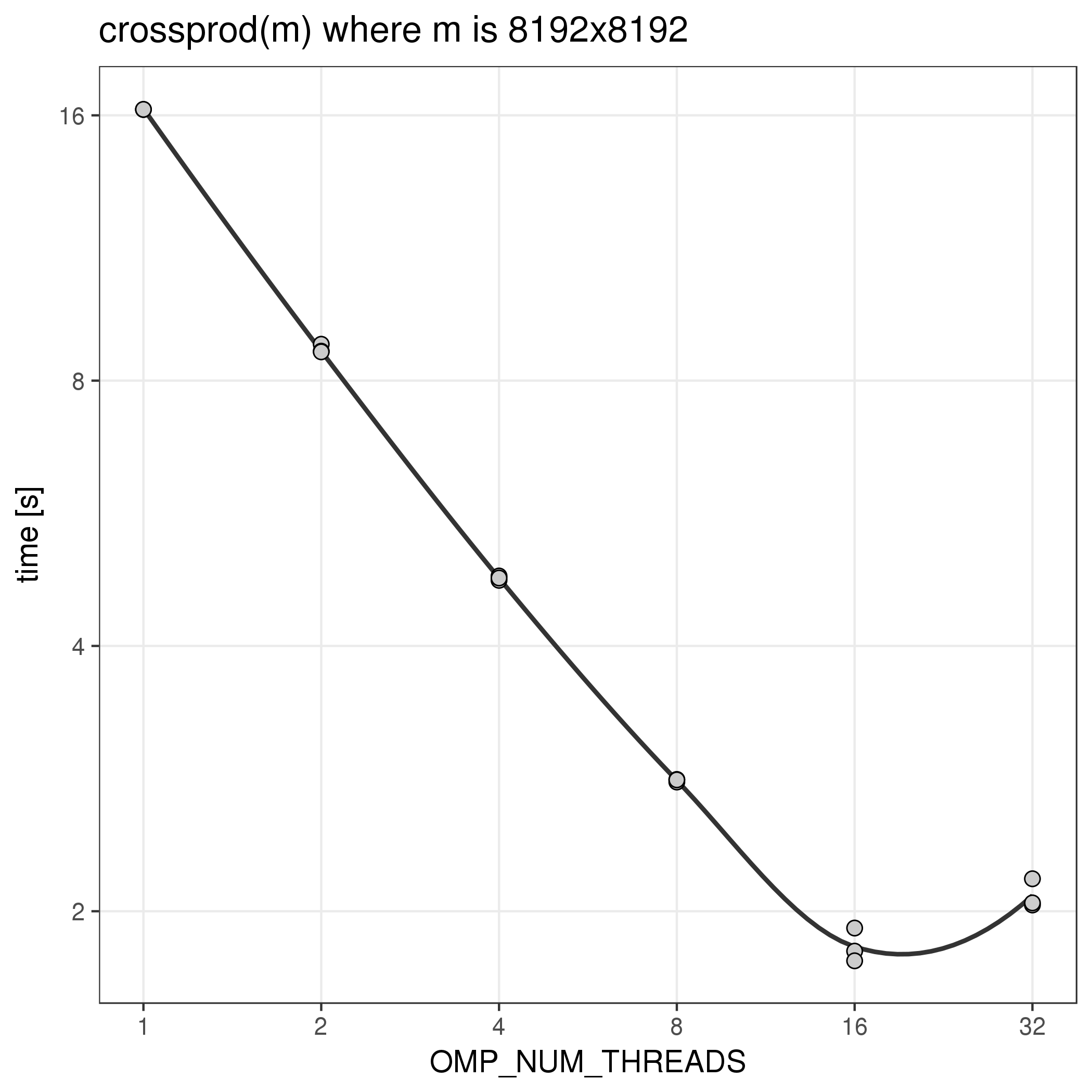
The function crossprod(m) which is equivalent to calculating
t(m) %*% m, for example, makes use of implicit parallelism in the
underlying math libraries and can benefit from using more than one thread. The number
of threads used by such functions is regulated by the environment variable
OMP_NUM_THREADS, which the R module sets automatically when
loaded as part of a batch or interactive job. Here is the runtime of
this function with different values for OMP_NUM_THREADS:
The code used for this benchmark was
# this file is benchmark2.R
runs <- 3
o <- 2^13
b <- 0

for (i in 1:runs) {
  a <- matrix(rnorm(o*o), o, o)
  invisible(gc())
  timing <- system.time({
    b <- crossprod(a)		# equivalent to: b <- t(a) %*% a
  })[3]
  cat(sprintf("%f\n", timing))
}
And was called with
node$ module load R/3.5
node$ OMP_NUM_THREADS=1 Rscript benchmark2.R
node$ OMP_NUM_THREADS=2 Rscript benchmark2.R
...
node$ OMP_NUM_THREADS=32 Rscript benchmark2.R
From within a job that had been allocated 32 CPUs.
Notes:
- The R wrapper sets
{OMP|MKL}_NUM_THREADS to 1.
This is done to avoid problems when also using explicit parallelism that
uses forked worker processes like for example the 'parallel' package. In that
case each worker may start OMP_NUM_THREADS threads so there
could be as many as ncpus * OMP_NUM_THREADS total threads. If
ncpus is set to the number of allocated CPUs, as would be the most common case,
that would lead to a huge overload of the job and could potentially fail
if the ulimit on the number of processes is exceeded.
- Increasing
OMP_NUM_THREADS and allocating more CPUs
may or may not increase performance of your code. Before running jobs
with more CPUs it is vital to benchmark single jobs and prove that
your code can benefit from implicit parallelism. Otherwise
resources will be wasted.
- Benchmarking is also important to measure efficiency of parallelism. Clearly,
in this example, running with more than 8 threads would be highly inefficient.
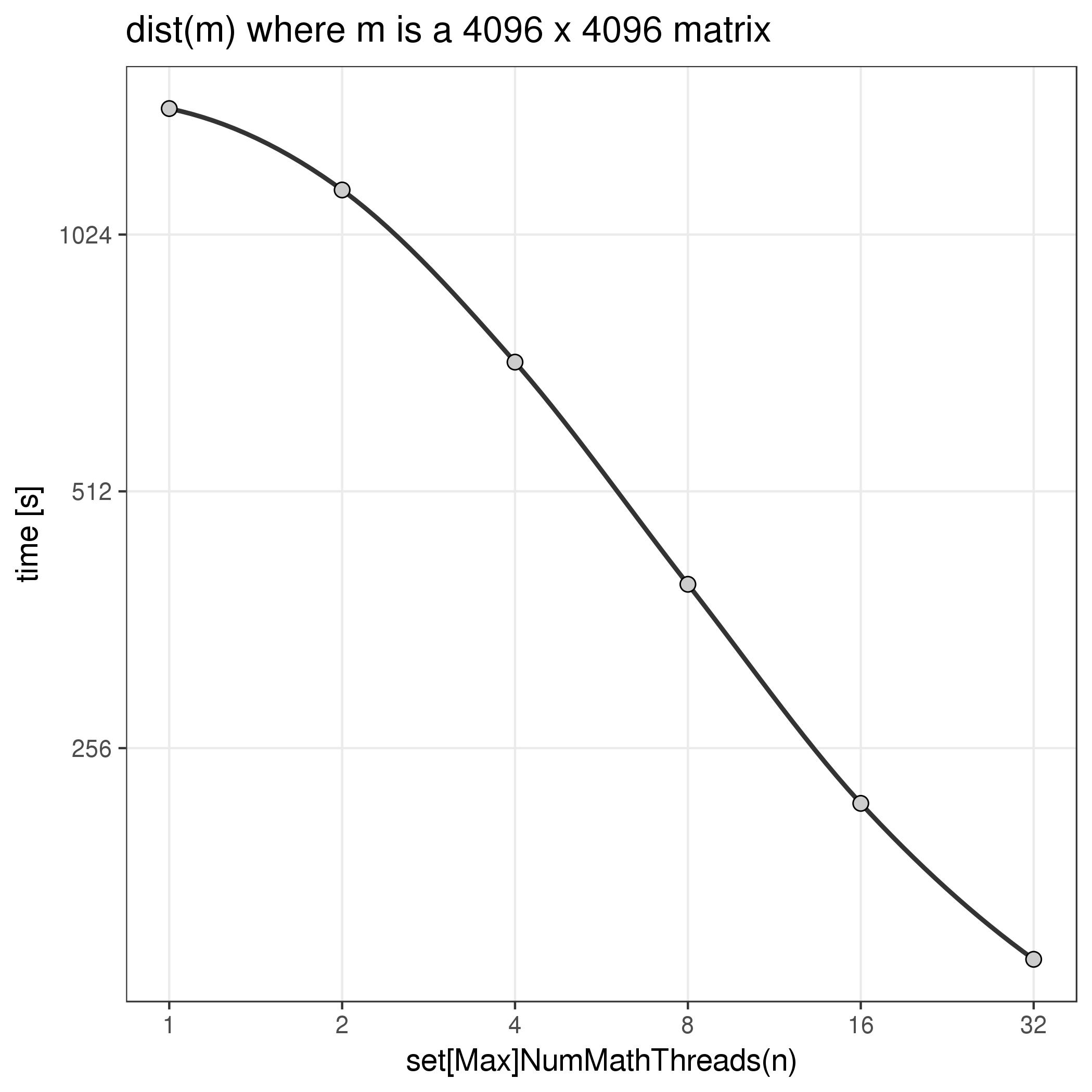
There appears to also be another level of parallelism within the R libraries.
One function that takes advantage of this is the dist function.
The level of parallelism allowed with this mechanism seems to be set with
two internal R functions (setMaxNumMathThreads and setNumMathThreads).
Note that this is a distinct mechanism - i.e. setting OMP_NUM_THREADS has
no impact on dist and setMaxNumMathThreads
has no impact on the performance of crossprod. Here is the performance
of dist with different numbers of threads:
The timings for this example were created with
# this file is benchmark1.R
rt <- data.frame()
o <- 2^12
m <- matrix(rnorm(o*o), o, o)
for (nt in c(1, 2, 4, 8, 16, 32)) {
    .Internal(setMaxNumMathThreads(nt))
    .Internal(setNumMathThreads(nt))
    res <- system.time(d <- dist(m))
    rt <- rbind(rt, c(nt, o, res[3]))
}
colnames(rt) <- c("threads", "order", "elapsed")
write.csv(rt, file="benchmark1.csv", row.names=F)
This was run within an allocation with 32 CPUs with
node$ OMP_NUM_THREADS=1 Rscript benchmark1.R
The same notes about benchmarking as above apply. Also note that there is
very little documentation about this to be found online.
Our R installations include the Rmpi and
pbdMPI interfaces to MPI (OpenMPI in our case). R/MPI code
can be run as batch jobs or from an sinteractive session with mpiexec or srun --mpi=pmix.
Running MPI code from an interactive R session is currently not supported.
The higher level snow MPI cluster interface is currently not supported. However,
the doMPI
parallel backend for foreach is supported.
See our MPI docs for more detail
Example Rmpi code
This is a lower level Rmpi script
# this script is test1.r
library(Rmpi)
id <- mpi.comm.rank(comm=0)
np <- mpi.comm.size (comm=0)
hostname <- mpi.get.processor.name()

msg <- sprintf ("Hello world from task %03d of %03d, on host %s \n", id , np , hostname)
cat(msg)

invisible(mpi.barrier(comm=0))
invisible(mpi.finalize())
It can be submitted as a batch job with the following script:
#! /bin/bash
# this script is test1.sh

module load R/4.1.0 || exit 1
srun --mpi=pmix Rscript test1.r
## or
# mpiexec Rscript test1.r
which would be submitted with
[user@biowulf]$ sbatch --ntasks=4 --nodes=2 --partition=multinode test1.sh
And would generate output similar to
Hello world from task 000 of 004, on host cn4101
Hello world from task 001 of 004, on host cn4102
Hello world from task 002 of 004, on host cn4103
Hello world from task 003 of 004, on host cn4104
Here is a Rmpi example with actual collective communication though still very simplistic.
This script derives an estimate for π in each task, gathers the results in task 0 and
repeats this process n times to arrive at a final estimate:
# this is test2.r
library(Rmpi)

# return a random number from /dev/urandom
readRandom <- function() {
  dev <- "/dev/urandom"
  rng = file(dev,"rb", raw=TRUE)
  n = readBin(rng, what="integer", 1) # read some 8-byte integers
  close(rng)
  return( n[1] ) # reduce range and shift
}

pi_dart <- function(i) {
    est <- mean(sqrt(runif(throws)^2 + runif(throws)^2) <= 1) * 4
    return(est)
}

id <- mpi.comm.rank(comm=0)
np <- mpi.comm.size (comm=0)
hostname <- mpi.get.processor.name()
rngseed <- readRandom()
cat(sprintf("This is task %03d of %03d, on host %s with seed %i\n",
    id , np , hostname, rngseed))
set.seed(rngseed)

throws <- 1e7
rounds <- 400
pi_global_sum = 0.0
for (i in 1:rounds) {
    # each task comes up with its own estimate of pi
    pi_est <- mean(sqrt(runif(throws)^2 + runif(throws)^2) <= 1) * 4
    # then we gather them all in task 0; type=2 means that the values are doubles
    pi_task_sum <- mpi.reduce(pi_est, type=2, op="sum", dest=0, comm=0)
    if (id == 0) {
        # task with id 0 then uses the sum to calculate an avarage across the
        # tasks and adds that to the global sum
        pi_global_sum <- pi_global_sum + (pi_task_sum / np)
    }
}

# when we're done, the task id 0 averages across all the rounds and prints the result
if (id == 0) {
    cat(sprintf("Real value of pi = %.10f\n", pi))
    cat(sprintf("  Estimate of pi = %.10f\n", pi_global_sum / rounds))
}

invisible(mpi.finalize())
Submitting this script with a batch script similar to the first example results
in output like this:
This is task 000 of 004, on host cn4101 with seed -303950071
This is task 001 of 004, on host cn4102 with seed -1074523673
This is task 002 of 004, on host cn4103 with seed 788983269
This is task 003 of 004, on host cn4104 with seed -922785662
Real value of pi = 3.1415926536
  Estimate of pi = 3.1415935438
doMPI example code
doMPI provides an MPI backend for the foreach package. Here is a simple hello-world-ish
doMPI example. Note that in my testing the least issues were encountered when
the foreach loops were run from the first rank of the MPI job.
suppressMessages({
    library(Rmpi)
    library(doMPI)
    library(foreach)
})

myrank <- mpi.comm.rank(comm=0)
cl <- doMPI::startMPIcluster()
registerDoMPI(cl)
if (myrank == 0) {
    cat("-------------------------------------------------\n")
    cat("== This is rank 0 running the foreach loops ==\n")


    x <- foreach(i=1:16, .combine="c") %dopar% {
        id <- mpi.comm.rank(comm=0)
        np <- mpi.comm.size (comm=0)
        hostname <- mpi.get.processor.name()
        sprintf ("Hello world from process %03d of %03d, on host %s \n", id , np , hostname)
    }
    print(x)

    x <- foreach(i=1:200, .combine="c") %dopar% {
        sqrt(i)
    }

    cat("-------------------------------------------------\n")
    print(x)

    x <- foreach(i=1:16, .combine="cbind") %dopar% {
        set.seed(i)
        rnorm(3)
    }


    cat("-------------------------------------------------\n")
    print(x)

}
closeCluster(cl)
mpi.quit(save="no")
Do not specify the number of tasks to run. doMPI clusters will hang during shutdown
if doMPI has to spawn worker processes. Instead, let mpiexec start the processes and then
doMPI will wire up a main process and workers from the existing processes. Note that the
startMPIcluster function has to be called early in the script for that reason.
Run a shiny app on biowulf
Shiny apps can be run on biowulf for a single user. Since they require tunneling a running
shiny app cannot be shared with other users. However, if the code for the app is accessible
to different users they each can run an ephemeral shiny app on biowulf. We will use the following
example application:
## this file is 01_hello.r
library(shiny)


ui <- fluidPage(

  # App title ----
  titlePanel("Hello Shiny!"),
  # Sidebar layout with input and output definitions ----
  sidebarLayout(
    # Sidebar panel for inputs ----
    sidebarPanel(
      # Input: Slider for the number of bins ----
      sliderInput(inputId = "bins",
                  label = "Number of bins:",
                  min = 1,
                  max = 50,
                  value = 30)
    ),
    # Main panel for displaying outputs ----
    mainPanel(
      # Output: Histogram ----
      plotOutput(outputId = "distPlot")
    )
  )
)

# Define server logic required to draw a histogram ----
server <- function(input, output) {
  # Histogram of the Old Faithful Geyser Data ----
  # with requested number of bins
  # This expression that generates a histogram is wrapped in a call
  # to renderPlot to indicate that:
  #
  # 1. It is "reactive" and therefore should be automatically
  #    re-executed when inputs (input$bins) change
  # 2. Its output type is a plot
  output$distPlot <- renderPlot({
    x    <- faithful$waiting
    bins <- seq(min(x), max(x), length.out = input$bins + 1)
    hist(x, breaks = bins, col = "#007bc2", border = "white",
         xlab = "Waiting time to next eruption (in mins)",
         main = "Histogram of waiting times")

    })
}

# which port to run on
port <- tryCatch(
  as.integer(Sys.getenv("PORT1", "none")),
  error = function(e) {
    cat("Please remember to use --tunnel to run a shiny app")
    cat("See https://hpc.nih.gov/docs/tunneling/")
    stop()
  }
)

# run the app
shinyApp(
  ui,
  server,
  options = list(port=port, launch.browser=F, host="127.0.0.1")
)
Start an sinteractive session with a tunnel
[user@biowulf]$ sinteractive --cpus-per-task=2 --mem=6g --gres=lscratch:10 --tunnel
salloc.exe: Pending job allocation 46116226
salloc.exe: job 46116226 queued and waiting for resources
salloc.exe: job 46116226 has been allocated resources
salloc.exe: Granted job allocation 46116226
salloc.exe: Waiting for resource configuration
salloc.exe: Nodes cn3144 are ready for job
[user@cn3144 ~]$ module load R
[user@cn3144 ~]$ Rscript 01_hello.r

Listening on http://127.0.0.1:34239
After you set up your tunnel you can use the URL above to access the shiny app.
Notes for individual packages
h2o
h2o is a machine learning package written in java. The R interface starts a java h2o instance
with a given number of threads and then connects to it through http. This fails on compute nodes
if the http proxy variables are set. Therefore it is necessary to unset http_proxy
before using h2o:
[user@biowulf]$ sinteractive --cpus-per-task=4 --mem=20g --gres=lscratch:10
salloc.exe: Pending job allocation 46116226
salloc.exe: job 46116226 queued and waiting for resources
salloc.exe: job 46116226 has been allocated resources
salloc.exe: Granted job allocation 46116226
salloc.exe: Waiting for resource configuration
salloc.exe: Nodes cn3144 are ready for job
[user@cn3144 ~]$ module load R/4.2
[user@cn3144 ~]$ unset http_proxy
[user@cn3144 ~]$ R
R version 4.2.0 (2022-04-22) -- "Vigorous Calisthenics"
Copyright (C) 2022 The R Foundation for Statistical Computing
Platform: x86_64-pc-linux-gnu (64-bit)

[...snip...]
> library(h2o)
> h2o.init(ip='localhost', nthreads=future::availableCores(), max_mem_size='12g')
H2O is not running yet, starting it now...

Note:  In case of errors look at the following log files:
    /tmp/RtmpVdW92Y/h2o_user_started_from_r.out
    /tmp/RtmpVdW92Y/h2o_user_started_from_r.err

openjdk version "1.8.0_161"
OpenJDK Runtime Environment (build 1.8.0_161-b14)
OpenJDK 64-Bit Server VM (build 25.161-b14, mixed mode)

Starting H2O JVM and connecting: . Connection successful!

R is connected to the H2O cluster:
    H2O cluster uptime:         1 seconds 683 milliseconds
    H2O cluster timezone:       America/New_York
    H2O data parsing timezone:  UTC
    H2O cluster version:        3.36.1.2
    H2O cluster version age:    3 months and 20 days !!!
    H2O cluster name:           H2O_started_from_R_user_ywu882
    H2O cluster total nodes:    1
    H2O cluster total memory:   10.64 GB
    H2O cluster total cores:    4
    H2O cluster allowed cores:  4
    H2O cluster healthy:        TRUE
    H2O Connection ip:          localhost
    H2O Connection port:        54321
    H2O Connection proxy:       NA
    H2O Internal Security:      FALSE
    R Version:                  R version 4.2.0 (2022-04-22)

>
dyno
dyno is a meta package that installs several other packages from the dynvers
(https://github.com/dynverse). It
includes some cran packages and some packages only available on github. We
generally don't install any new github-only R packages any more so here are the
instructions for installing this as a user.
Installation
###
### 1. install with the default dependent packages
###
[user@biowulf]$ sinteractive --gres=lscratch:5
salloc.exe: Pending job allocation 46116226
salloc.exe: job 46116226 queued and waiting for resources
salloc.exe: job 46116226 has been allocated resources
salloc.exe: Granted job allocation 46116226
salloc.exe: Waiting for resource configuration
salloc.exe: Nodes cn3144 are ready for job
[user@cn3144 ~]$ module load R/4.2
[user@cn3144 ~]$ R -q --no-save --no-restore -e 'devtools::install_github("dynverse/dyno")'

###
### 2. install a pached version of babelwhale
###
[user@cn3144 ~]$ git clone https://github.com/dynverse/babelwhale.git
[user@cn3144 ~]$ patch -p0 <<'__EOF__'
--- babelwhale/R/run.R.orig     2021-07-16 20:58:26.563714000 -0400
+++ babelwhale/R/run.R  2021-07-16 20:58:26.483721000 -0400
@@ -122,6 +122,8 @@
         environment_variables %>% gsub("^.*=", "", .),
         environment_variables %>% gsub("^(.*)=.*$", "SINGULARITYENV_\\1", .)
       ),
+      "http_proxy" = Sys.getenv("http_proxy"),
+      "https_proxy" = Sys.getenv("https_proxy"),
       "SINGULARITY_TMPDIR" = tmpdir,
       "SINGULARITY_CACHEDIR" = config$cache_dir,
       "PATH" = Sys.getenv("PATH") # pass the path along
__EOF__

[user@cn3144 ~]$ R CMD INSTALL babelwhale

###
### 3. Create a configuration that uses a dedicated singularity cache somewhere
###    outside the home directory. In this example using `/data/$USER/dynocache`
###

[user@cn3144 ~]$ R -q --no-save --no-restore <<'__EOF__'
config <- babelwhale::create_singularity_config(
  cache_dir = "/data/$USER/dynocache"
)
babelwhale::set_default_config(config, permanent = TRUE)
__EOF__
Notes:
- There is a bug in the `plot_dimred` function - see
https://github.com/dynverse/dynplot/issues/54. I tried installing
the devel version but it didn't help. YMMV
- If you want to use the parts that use shiny (e.g. guidelines_shiny)
you will need to use a tunnel and call the function like
guidelines_shiny(dataset, port=####, launch.browser=F) where
#### is the port set up by the `sinteractive --tunnel`